Chapter 8. Inferene Engines¶

import os
import warnings

import arviz as az
import matplotlib.pyplot as plt
import pandas as pd
import seaborn as sns

import jax.numpy as jnp
from jax import random, vmap, local_device_count, pmap, lax, tree_map, hessian
from jax import nn as jnn
from jax.scipy import stats, special

import numpyro
import numpyro.distributions as dist
import numpyro.optim as optim

from numpyro.infer import MCMC, NUTS, HMC, Predictive
from numpyro.diagnostics import hpdi, print_summary
from numpyro.infer import Predictive, SVI, Trace_ELBO, init_to_value
from numpyro.infer.autoguide import AutoLaplaceApproximation

seed=1234

if "SVG" in os.environ:
    %config InlineBackend.figure_formats = ["svg"]
warnings.formatwarning = lambda message, category, *args, **kwargs: "{}: {}\n".format(
    category.__name__, message
)
az.style.use("arviz-darkgrid")
numpyro.set_platform("cpu") # or "gpu", "tpu" depending on system
numpyro.set_host_device_count(local_device_count())

# import pymc3 as pm
# import numpy as np
# import pandas as pd
# import scipy.stats as stats
# import matplotlib.pyplot as plt
# import arviz as az

# az.style.use('arviz-darkgrid')

Non-Markovian methods¶

Grid computing¶

def posterior_grid(grid_points=50, heads=6, tails=9):
    """ 
    A grid implementation for the coin-flipping problem 
    """
    grid = jnp.linspace(0.01, 1, grid_points)
    prior = jnp.repeat(1/grid_points, grid_points)  # uniform prior
    likelihood = jnp.exp(dist.Binomial(total_count=(heads+tails), probs=grid).log_prob(heads))
    posterior = likelihood * prior
    posterior /= posterior.sum()
    return grid, posterior

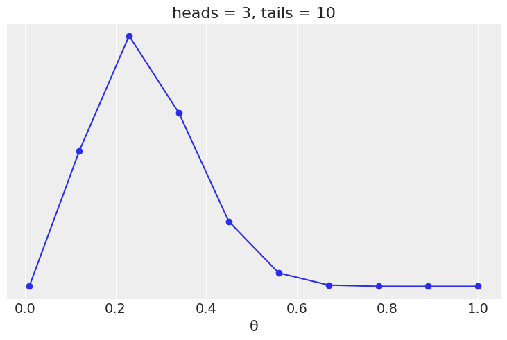
Assuming we flip a coin 13 times and we observed 3 head we have:

data = jnp.repeat(jnp.array([0, 1]), jnp.asarray((10, 3)))
points = 10
h = data.sum()
t = len(data) - h
grid, posterior = posterior_grid(points, h, t) 

plt.plot(grid, posterior, 'o-')

plt.title(f'heads = {h}, tails = {t}')
plt.yticks([])
plt.xlabel('θ');

../_images/08-inference-engines_7_0.png

Quadratic method¶

def model(obs=None):
    p = numpyro.sample('p', dist.Beta(concentration1=1., concentration0=1.))
    w = numpyro.sample('w', dist.Binomial(total_count=1, probs=p), obs=obs)
                       
guide = AutoLaplaceApproximation(model)
svi = SVI(model, guide, optim.Adam(1), Trace_ELBO(), obs=data)
svi_result = svi.run(random.PRNGKey(0), 20000)
params = svi_result.params
params

100%|████████████████████| 20000/20000 [00:01<00:00, 11830.65it/s, init loss: 11.2695, avg. loss [19001-20000]: 8.6997]

{'auto_loc': DeviceArray([-1.0116092], dtype=float32)}

samples = guide.sample_posterior(random.PRNGKey(0), params, (10000,))

xs = jnp.sort(samples['p'])
std_q = jnp.std(xs)
mean_q = jnp.mean(xs)
mean_q, std_q 

(DeviceArray(0.28205067, dtype=float32),
 DeviceArray(0.11372714, dtype=float32))

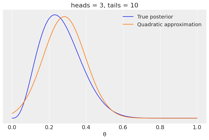
# analytical calculation
x = jnp.linspace(0, 1, 100)
plt.plot(x, jnp.exp(dist.Beta(h+1, t+1).log_prob(x)), label='True posterior')

# quadratic approximation
plt.plot(x, jnp.exp(dist.Normal(mean_q, std_q).log_prob(x)),label='Quadratic approximation')
# plt.plot(x, guide.(params).sample(random.PRNGKey(0), sample_shape=(len(x),)))
plt.legend(loc=0, fontsize=13)

plt.title(f'heads = {h}, tails = {t}')
plt.xlabel('θ', fontsize=14)
plt.yticks([])

([], [])

../_images/08-inference-engines_12_1.png

quantiles = guide.quantiles(params, 0.5)
quantiles

{'p': DeviceArray(0.26666504, dtype=float32)}

guide.median(params)

{'p': DeviceArray(0.26666504, dtype=float32)}

# predictive = Predictive(guide, params=params, num_samples=1000)
# samples = predictive(random.PRNGKey(1), data)

numpyro.diagnostics.hpdi(samples['p'], prob=0.5)

array([0.17510453, 0.32284716], dtype=float32)

# with pm.Model() as normal_aproximation:
#     p = pm.Beta('p', 1., 1.)
#     w = pm.Binomial('w',n=1, p=p, observed=data)
#     mean_q = pm.find_MAP()
#     std_q = ((1/pm.find_hessian(mean_q, vars=[p]))**0.5)[0]
# mean_q['p'], std_q

Markovian methods¶

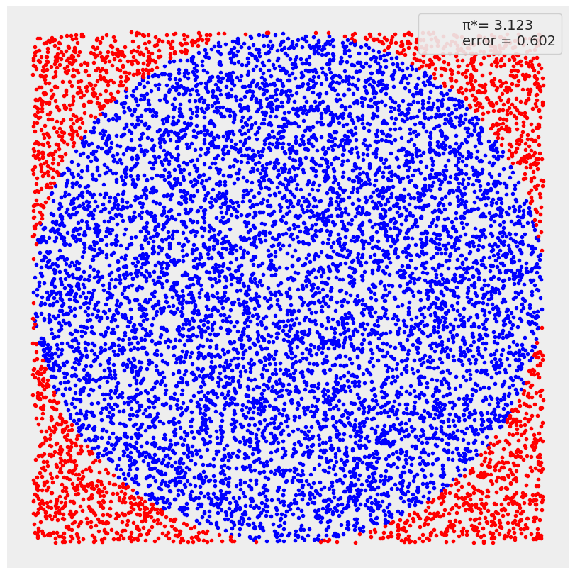
Monte Carlo¶

N = 10000

x, y = dist.Uniform(low=-1, high=1).sample(random.PRNGKey(0), sample_shape=(2, N))
inside = (x**2 + y**2) <= 1
pi = inside.sum()*4/N
error = abs((pi - jnp.pi) / pi) * 100
 
outside = jnp.invert(inside)
 
plt.figure(figsize=(8, 8))
plt.plot(x[inside], y[inside], 'b.')
plt.plot(x[outside], y[outside], 'r.')
plt.plot(0, 0, label=f'π*= {pi:4.3f}\nerror = {error:4.3f}', alpha=0)
plt.axis('square')
plt.xticks([])
plt.yticks([])
plt.legend(loc=1, frameon=True, framealpha=0.9)

<matplotlib.legend.Legend at 0x7ffb946d5be0>

../_images/08-inference-engines_19_1.png

def metropolis(func, draws=10000):
    """A very simple Metropolis implementation"""
    trace = jnp.zeros(draws)
    old_x = 0.5  # func.mean()
    old_prob = jnp.exp(func.log_prob(old_x))

    delta = dist.Normal(loc=0, scale=0.5).sample(random.PRNGKey(0), sample_shape=(draws,))
    for i in range(draws):
        new_x = old_x + delta[i]
        new_prob = jnp.exp(func.log_prob(new_x))
        acceptance = new_prob / old_prob
#         if acceptance >= dist.Uniform(low=0, high=1).sample(random.PRNGKey(i)):
        if acceptance >= random.uniform(random.PRNGKey(i)):
            trace = trace.at[i].set(new_x)
            old_x = new_x
            old_prob = new_prob
        else:
            # x[idx] = y``, use ``x = x.at[idx].set(y)
            trace = trace.at[i].set(old_x)

    return trace

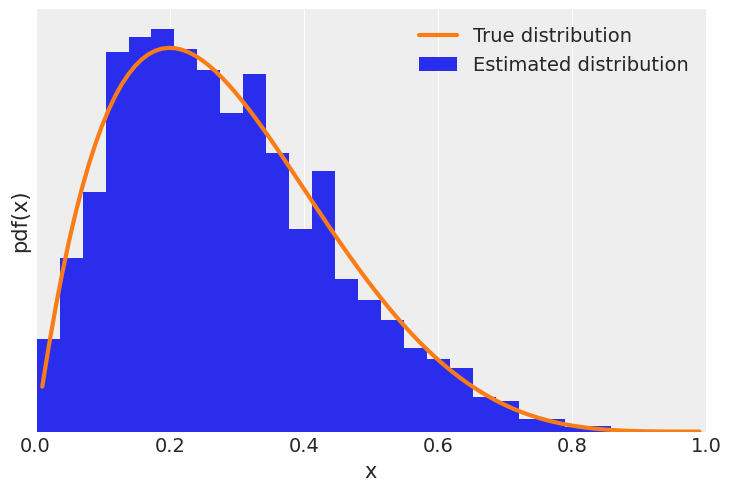
func = dist.Beta(concentration1=2, concentration0=5)

trace = metropolis(func=func) 
x = jnp.linspace(0.01, .99, 100) 
y = jnp.exp(func.log_prob(x)) 
plt.xlim(0, 1) 
plt.plot(x, y, 'C1-', lw=3, label='True distribution') 
plt.hist(trace[trace > 0], bins=25, density=True, label='Estimated distribution') 
plt.xlabel('x') 
plt.ylabel('pdf(x)')
plt.yticks([]) 
plt.legend()

<matplotlib.legend.Legend at 0x7ffb7765be50>

../_images/08-inference-engines_21_1.png

Diagnosing the samples¶

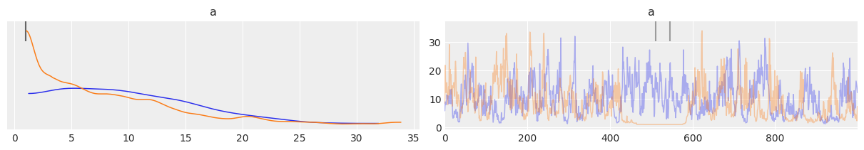
def centered_model(obs=None):
    a = numpyro.sample('a', dist.HalfNormal(scale=10))
    b = numpyro.sample('b', dist.Normal(loc=0, scale=a), sample_shape=(10,))
    
kernel = NUTS(centered_model, target_accept_prob=0.85)
trace_cm = MCMC(kernel, num_warmup=1000, num_samples=1000, num_chains=2, chain_method='sequential')
trace_cm.run(random.PRNGKey(seed))

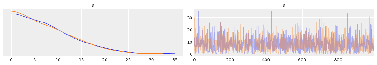
def non_centered_model(obs=None):
    a = numpyro.sample('a', dist.HalfNormal(scale=10))
    b_offset = numpyro.sample('b_offset', dist.Normal(loc=0, scale=1), sample_shape=(10,))
    b = numpyro.deterministic('b', 0 + b_offset * a)
    
kernel = NUTS(non_centered_model, target_accept_prob=0.85)
trace_ncm = MCMC(kernel, num_warmup=1000, num_samples=1000, num_chains=2, chain_method='sequential')
trace_ncm.run(random.PRNGKey(seed))

sample: 100%|██████████████████████████| 2000/2000 [00:02<00:00, 794.15it/s, 31 steps of size 2.11e-01. acc. prob=0.92]
sample: 100%|██████████████████████████| 2000/2000 [00:00<00:00, 6585.73it/s, 7 steps of size 1.84e-01. acc. prob=0.81]
sample: 100%|███████████████████████████| 2000/2000 [00:02<00:00, 858.42it/s, 7 steps of size 3.92e-01. acc. prob=0.92]
sample: 100%|██████████████████████████| 2000/2000 [00:00<00:00, 7252.10it/s, 7 steps of size 5.03e-01. acc. prob=0.89]

az.plot_trace(trace_cm, var_names=['a'], divergences='top', compact=False)

array([[<AxesSubplot:title={'center':'a'}>,
        <AxesSubplot:title={'center':'a'}>]], dtype=object)

../_images/08-inference-engines_24_1.png

az.plot_trace(trace_ncm, var_names=['a'], compact=False)

array([[<AxesSubplot:title={'center':'a'}>,
        <AxesSubplot:title={'center':'a'}>]], dtype=object)

../_images/08-inference-engines_25_1.png

az.summary(trace_cm)

	mean	sd	hdi_3%	hdi_97%	mcse_mean	mcse_sd	ess_bulk	ess_tail	r_hat
a	9.190	6.295	1.013	20.570	0.749	0.532	41.0	22.0	1.05
b[0]	0.052	11.401	-24.873	20.704	0.226	0.359	2342.0	771.0	1.02
b[1]	0.247	10.922	-23.837	21.836	0.214	0.365	2497.0	936.0	1.02
b[2]	0.039	10.862	-21.110	21.709	0.216	0.362	2675.0	928.0	1.03
b[3]	-0.065	11.525	-22.748	23.628	0.215	0.402	2880.0	998.0	1.02
b[4]	0.045	11.595	-23.655	22.588	0.221	0.356	3088.0	825.0	1.02
b[5]	0.340	10.935	-19.502	22.569	0.217	0.399	2521.0	802.0	1.02
b[6]	0.217	12.287	-26.847	23.079	0.251	0.432	2750.0	715.0	1.03
b[7]	0.366	11.802	-26.457	21.237	0.219	0.366	2806.0	996.0	1.03
b[8]	0.381	11.643	-20.940	24.580	0.226	0.338	2814.0	988.0	1.05
b[9]	0.145	10.404	-19.198	21.812	0.183	0.281	3271.0	1080.0	1.01

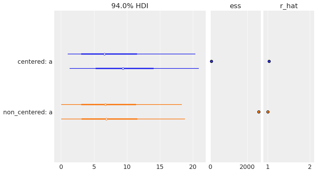
az.rhat(trace_cm)['a'].values, az.rhat(trace_ncm)['a'].values

(array(1.04987792), array(1.00006256))

az.plot_forest([trace_cm, trace_ncm], model_names=['centered', 'non_centered'],
               var_names=['a'], r_hat=True, ess=True)

array([<AxesSubplot:title={'center':'94.0% HDI'}>,
       <AxesSubplot:title={'center':'ess'}>,
       <AxesSubplot:title={'center':'r_hat'}>], dtype=object)

../_images/08-inference-engines_28_1.png

summaries = pd.concat([az.summary(trace_cm, var_names=['a']),
           az.summary(trace_ncm, var_names=['a'])])
summaries.index = ['centered', 'non_centered']
summaries

	mean	sd	hdi_3%	hdi_97%	mcse_mean	mcse_sd	ess_bulk	ess_tail	r_hat
centered	9.190	6.295	1.013	20.570	0.749	0.532	41.0	22.0	1.05
non_centered	7.896	6.012	0.007	18.599	0.117	0.083	1567.0	727.0	1.00

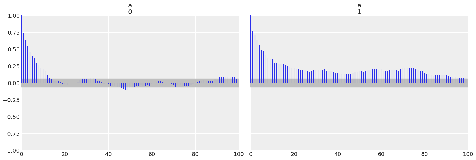
az.plot_autocorr(trace_cm, var_names=['a'])

array([<AxesSubplot:title={'center':'a\n0'}>,
       <AxesSubplot:title={'center':'a\n1'}>], dtype=object)

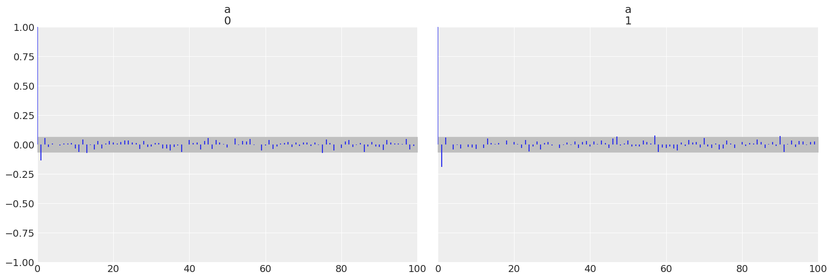
../_images/08-inference-engines_30_1.png

az.plot_autocorr(trace_ncm, var_names=['a'])

array([<AxesSubplot:title={'center':'a\n0'}>,
       <AxesSubplot:title={'center':'a\n1'}>], dtype=object)

../_images/08-inference-engines_31_1.png

Effective sample size¶

az.ess(trace_cm)['a'].values

array(41.46579247)

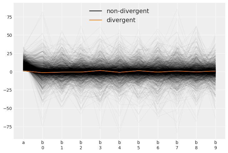
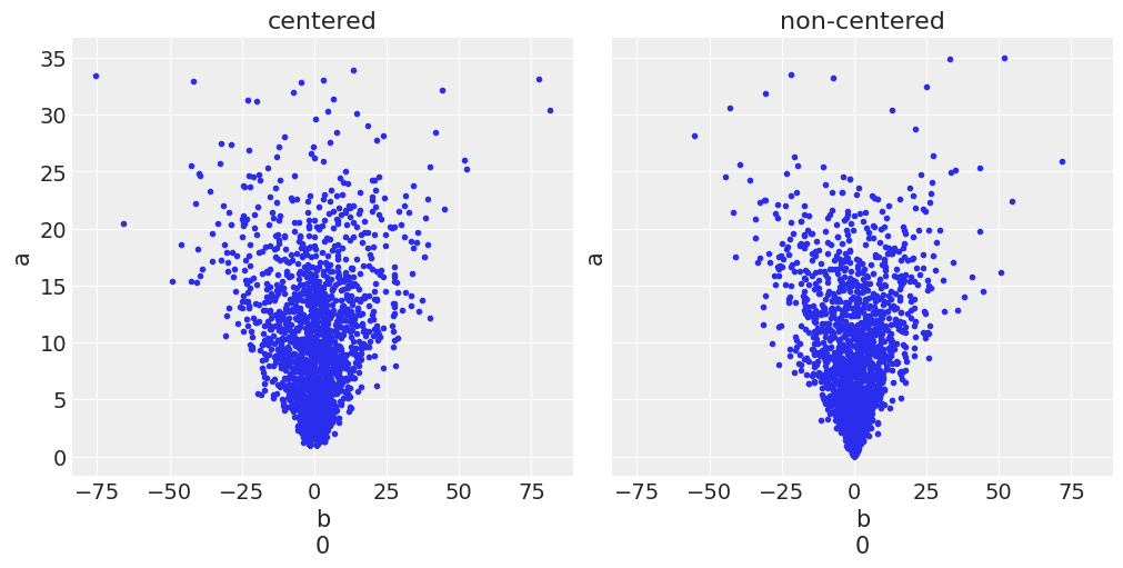
Divergences¶

_, ax = plt.subplots(1, 2, sharey=True, sharex=True, figsize=(10, 5), constrained_layout=True)

for idx, tr in enumerate([trace_cm, trace_ncm]):
    az.plot_pair(tr, var_names=['b', 'a'], coords={'b_dim_0':[0]}, kind='scatter',
                 divergences=True, contour=False, divergences_kwargs={'color':'C1'},
                 ax=ax[idx])
    ax[idx].set_title(['centered', 'non-centered'][idx])

UserWarning: Divergences data not found, plotting without divergences. Make sure the sample method provides divergences data and that it is present in the `diverging` field of `sample_stats` or `sample_stats_prior` or set divergences=False
UserWarning: Divergences data not found, plotting without divergences. Make sure the sample method provides divergences data and that it is present in the `diverging` field of `sample_stats` or `sample_stats_prior` or set divergences=False

../_images/08-inference-engines_35_1.png

az.plot_parallel(trace_cm)

<AxesSubplot:>

../_images/08-inference-engines_36_1.png

previous

Chapter 7. Gaussian Processes

next

Chapter 1 Exercises