
Chapter 4. Generalizing Linear Models
import os
import warnings

import arviz as az
import matplotlib.pyplot as plt
import pandas as pd
import seaborn as sns

import jax.numpy as jnp
from jax import random, vmap, local_device_count, pmap
from jax import nn as jnn

import numpyro
import numpyro.distributions as dist
import numpyro.optim as optim

from numpyro.infer import MCMC, NUTS, HMC, Predictive
from numpyro.diagnostics import hpdi, print_summary
from numpyro.infer import Predictive, SVI, Trace_ELBO, init_to_value
from numpyro.infer.autoguide import AutoLaplaceApproximation


seed=1234

if "SVG" in os.environ:
    %config InlineBackend.figure_formats = ["svg"]
warnings.formatwarning = lambda message, category, *args, **kwargs: "{}: {}\n".format(
    category.__name__, message
)
az.style.use("arviz-darkgrid")
numpyro.set_platform("cpu") # or "gpu", "tpu" depending on system
numpyro.set_host_device_count(local_device_count())
# import pymc3 as pm
# import numpy as np
# import pandas as pd
# import theano.tensor as tt
# import seaborn as sns
# import scipy.stats as stats
# from scipy.special import expit as logistic
# import matplotlib.pyplot as plt
# import arviz as az
# az.style.use('arviz-darkgrid')
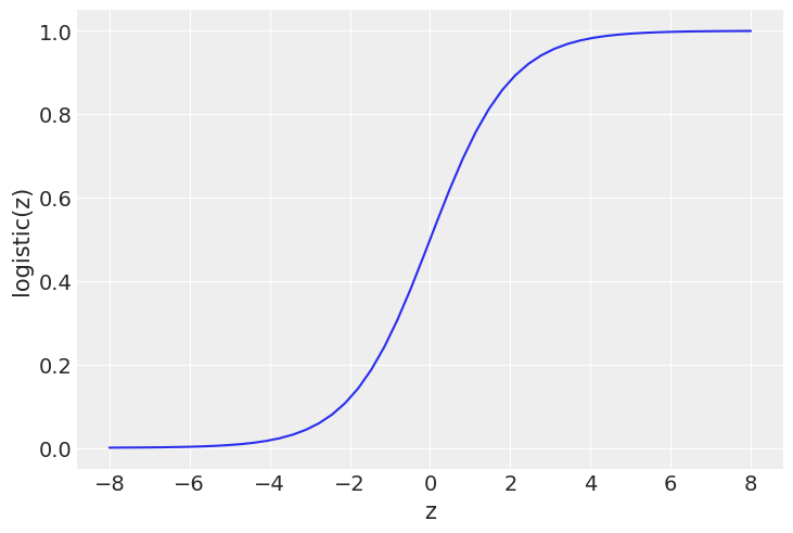
Logistic regression
z = jnp.linspace(-8, 8)
plt.plot(z, 1 / (1 + jnp.exp(-z)))
plt.xlabel('z')
plt.ylabel('logistic(z)')
Text(0, 0.5, 'logistic(z)')
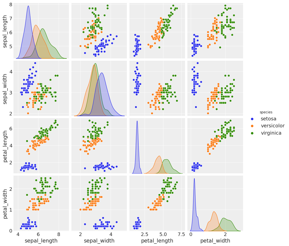
The iris dataset
iris = pd.read_csv('../data/iris.csv')
iris.head()
| sepal_length | sepal_width | petal_length | petal_width | species | |
|---|---|---|---|---|---|
| 0 | 5.1 | 3.5 | 1.4 | 0.2 | setosa |
| 1 | 4.9 | 3.0 | 1.4 | 0.2 | setosa |
| 2 | 4.7 | 3.2 | 1.3 | 0.2 | setosa |
| 3 | 4.6 | 3.1 | 1.5 | 0.2 | setosa |
| 4 | 5.0 | 3.6 | 1.4 | 0.2 | setosa |
sns.stripplot(x="species", y="sepal_length", data=iris, jitter=True)
<AxesSubplot:xlabel='species', ylabel='sepal_length'>

sns.pairplot(iris, hue='species', diag_kind='kde')
UserWarning: This figure was using constrained_layout, but that is incompatible with subplots_adjust and/or tight_layout; disabling constrained_layout.
<seaborn.axisgrid.PairGrid at 0x12f0f98b0>
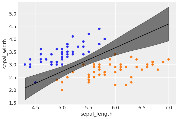
The logistic model applied to the iris dataset
df = iris.query("species == ('setosa', 'versicolor')")
y_0 = pd.Categorical(df['species']).codes
x_n = 'sepal_length'
x_0 = df[x_n].values
x_c = x_0 - x_0.mean()
def model(obs=None):
    α = numpyro.sample('α', dist.Normal(loc=0, scale=10))
    β = numpyro.sample('β', dist.Normal(loc=0, scale=1))
    ϵ = numpyro.sample('ϵ', dist.HalfCauchy(scale=5))

    μ = α + jnp.dot(x_c, β)
    θ = numpyro.deterministic('θ', jnn.sigmoid(μ))
    bd = numpyro.deterministic('bd', -α/β)

    yl = numpyro.sample('yl', dist.Bernoulli(probs=θ), obs=obs)


kernel = NUTS(model)
mcmc = MCMC(kernel, num_warmup=5000, num_samples=5000, num_chains=4, chain_method='sequential')
mcmc.run(random.PRNGKey(seed), obs=y_0)
sample: 100%|████████████████████████| 10000/10000 [00:04<00:00, 2410.92it/s, 3 steps of size 7.02e-01. acc. prob=0.91]
sample: 100%|████████████████████████| 10000/10000 [00:05<00:00, 1991.31it/s, 3 steps of size 7.69e-01. acc. prob=0.88]
sample: 100%|████████████████████████| 10000/10000 [00:01<00:00, 6316.56it/s, 3 steps of size 7.60e-01. acc. prob=0.89]
sample: 100%|████████████████████████| 10000/10000 [00:01<00:00, 5977.72it/s, 3 steps of size 6.80e-01. acc. prob=0.91]
varnames = ['α', 'β', 'bd']
az.summary(mcmc, varnames)
| mean | sd | hdi_3% | hdi_97% | mcse_mean | mcse_sd | ess_bulk | ess_tail | r_hat | |
|---|---|---|---|---|---|---|---|---|---|
| α | 0.134 | 0.273 | -0.395 | 0.631 | 0.002 | 0.002 | 16846.0 | 14060.0 | 1.0 |
| β | 3.255 | 0.542 | 2.237 | 4.254 | 0.004 | 0.003 | 16426.0 | 13782.0 | 1.0 |
| bd | -0.040 | 0.085 | -0.204 | 0.116 | 0.001 | 0.001 | 17877.0 | 14539.0 | 1.0 |
# az.plot_trace(mcmc, compact=False)
jnp.squeeze(dist.Normal(y_0, 0.02).sample(random.PRNGKey(0), (1,)), axis=0).shape, x_c.shape
((100,), (100,))
theta = mcmc.get_samples()['θ'].mean(axis=0)
idx = jnp.argsort(x_c)
plt.plot(x_c[idx], theta[idx], color='C2', lw=3)

plt.vlines(mcmc.get_samples()['bd'].mean(), 0, 1, color='k')

bd_hdi = az.hdi(mcmc.get_samples()['bd'].copy())
plt.fill_betweenx([0, 1], bd_hdi[0], bd_hdi[1], color='k', alpha=0.5)

plt.scatter(x_c, jnp.squeeze(dist.Normal(y_0, 0.02).sample(random.PRNGKey(0), (1,)), axis=0),
            marker='.', color=[f'C{x}' for x in y_0])
az.plot_hdi(x_c, mcmc.get_samples()['θ'], color='C2')

plt.xlabel(x_n)
plt.ylabel('θ', rotation=0)
# use original scale for xticks
locs, _ = plt.xticks()
plt.xticks(locs, jnp.round(locs + x_0.mean(), 1))
FutureWarning: hdi currently interprets 2d data as (draw, shape) but this will change in a future release to (chain, draw) for coherence with other functions
([<matplotlib.axis.XTick at 0x131fc7f40>,
  <matplotlib.axis.XTick at 0x131fc7f10>,
  <matplotlib.axis.XTick at 0x131c052e0>,
  <matplotlib.axis.XTick at 0x131e97c40>,
  <matplotlib.axis.XTick at 0x131e977f0>,
  <matplotlib.axis.XTick at 0x131e979a0>,
  <matplotlib.axis.XTick at 0x131e87bb0>,
  <matplotlib.axis.XTick at 0x131e42100>],
 [Text(-1.5, 0, '4.0'),
  Text(-1.0, 0, '4.5'),
  Text(-0.5, 0, '5.0'),
  Text(0.0, 0, '5.5'),
  Text(0.5, 0, '6.0'),
  Text(1.0, 0, '6.5'),
  Text(1.5, 0, '7.0'),
  Text(2.0, 0, '7.5')])

Multiple logistic regression
df = iris.query("species == ('setosa', 'versicolor')")
y_1 = pd.Categorical(df['species']).codes
x_n = ['sepal_length', 'sepal_width']
x_1 = df[x_n].values
def model(obs=None):
    α = numpyro.sample('α', dist.Normal(loc=0, scale=10))
    β = numpyro.sample('β', dist.Normal(loc=0, scale=2), sample_shape=(len(x_n),))

    μ = α + jnp.dot(x_1, β)
    θ = numpyro.deterministic('θ', 1 / (1 + jnp.exp(-μ)))
    bd = numpyro.deterministic('bd', -α/β[1] - β[0]/β[1] * x_1[:,0])

    yl = numpyro.sample('yl', dist.Bernoulli(probs=θ), obs=obs)


kernel = NUTS(model)
mcmc2 = MCMC(kernel, num_warmup=5000, num_samples=5000, num_chains=2, chain_method='sequential')
mcmc2.run(random.PRNGKey(seed), obs=y_1)
sample: 100%|███████████████████████| 10000/10000 [00:06<00:00, 1447.78it/s, 19 steps of size 6.53e-02. acc. prob=0.93]
sample: 100%|███████████████████████| 10000/10000 [00:01<00:00, 5115.02it/s, 63 steps of size 5.24e-02. acc. prob=0.95]
varnames = ['α', 'β']
az.plot_forest(mcmc2, var_names=varnames);

idx = jnp.argsort(x_1[:,0])
bd = mcmc2.get_samples()['bd'].mean(0)[idx]
plt.scatter(x_1[:,0], x_1[:,1], c=[f'C{x}' for x in y_0])
plt.plot(x_1[:,0][idx], bd, color='k');

az.plot_hdi(x_1[:,0], mcmc2.get_samples()['bd'], color='k')

plt.xlabel(x_n[0])
plt.ylabel(x_n[1])
FutureWarning: hdi currently interprets 2d data as (draw, shape) but this will change in a future release to (chain, draw) for coherence with other functions
Text(0, 0.5, 'sepal_width')
Interpreting the coefficients of a logistic regression
probability = jnp.linspace(0.01, 1, 100)
odds = probability / (1 - probability)

_, ax1 = plt.subplots()
ax2 = ax1.twinx()
ax1.plot(probability, odds, 'C0')
ax2.plot(probability, jnp.log(odds), 'C1')

ax1.set_xlabel('probability')
ax1.set_ylabel('odds', color='C0')
ax2.set_ylabel('log-odds', color='C1')
ax1.grid(False)
ax2.grid(False)

df = az.summary(mcmc2, var_names=varnames)
df
| mean | sd | hdi_3% | hdi_97% | mcse_mean | mcse_sd | ess_bulk | ess_tail | r_hat | |
|---|---|---|---|---|---|---|---|---|---|
| α | -9.294 | 4.668 | -18.053 | -0.598 | 0.087 | 0.062 | 2878.0 | 3643.0 | 1.0 |
| β[0] | 4.696 | 0.882 | 3.088 | 6.368 | 0.017 | 0.012 | 2651.0 | 3243.0 | 1.0 |
| β[1] | -5.185 | 0.981 | -7.025 | -3.437 | 0.016 | 0.012 | 3727.0 | 4204.0 | 1.0 |
from jax.scipy.special import expit as logistic

x_1 = 4.5  # sepal_length
x_2 = 3   # sepal_width

log_odds_versicolor_i = (df['mean'] * [1, x_1, x_2]).sum()
probability_versicolor_i = logistic(log_odds_versicolor_i)


log_odds_versicolor_f = (df['mean'] * [1, x_1 + 1, x_2]).sum()
probability_versicolor_f = logistic(log_odds_versicolor_f)

log_odds_versicolor_f - log_odds_versicolor_i, probability_versicolor_f - probability_versicolor_i
(4.6960000000000015, DeviceArray(0.7031797, dtype=float32))
Dealing with correlated variables
corr = iris[iris['species'] != 'virginica'].corr()
mask = jnp.tri(*corr.shape).T
type(mask.copy())
numpy.ndarray
jnp.abs(jnp.asarray(corr))
DeviceArray([[1.        , 0.20592576, 0.81245786, 0.78960824],
             [0.20592576, 1.        , 0.6026631 , 0.5708832 ],
             [0.81245786, 0.6026631 , 1.        , 0.9793217 ],
             [0.78960824, 0.5708832 , 0.9793217 , 1.        ]],            dtype=float32)
sns.heatmap(jnp.abs(jnp.asarray(corr)), mask=mask.copy(), annot=True, cmap='viridis')
<AxesSubplot:>

Dealing with unbalanced classes
df = iris.query("species == ('setosa', 'versicolor')")
df = df[45:]
y_3 = pd.Categorical(df['species']).codes
x_n = ['sepal_length', 'sepal_width']
x_3 = df[x_n].values
def model(obs=None):
    α = numpyro.sample('α', dist.Normal(loc=0, scale=10))
    β = numpyro.sample('β', dist.Normal(loc=0, scale=2), sample_shape=(len(x_n),))

    μ = α + jnp.dot(x_3, β)
    θ = numpyro.deterministic('θ', 1 / (1 + jnp.exp(-μ)))
    bd = numpyro.deterministic('bd', -α/β[1] - β[0]/β[1] * x_3[:,0])

    yl = numpyro.sample('yl', dist.Bernoulli(probs=θ), obs=obs)


kernel = NUTS(model)
mcmc3 = MCMC(kernel, num_warmup=500, num_samples=1000, num_chains=2, chain_method='sequential')
mcmc3.run(random.PRNGKey(seed), obs=y_3)
sample: 100%|██████████████████████████| 1500/1500 [00:06<00:00, 241.92it/s, 63 steps of size 6.37e-02. acc. prob=0.93]
sample: 100%|█████████████████████████| 1500/1500 [00:00<00:00, 4949.02it/s, 63 steps of size 6.91e-02. acc. prob=0.95]
az.plot_trace(mcmc3, varnames);

idx = jnp.argsort(x_3[:,0])
bd = mcmc3.get_samples()['bd'].mean(0)[idx]
plt.scatter(x_3[:,0], x_3[:,1], c= [f'C{x}' for x in y_3])
plt.plot(x_3[:,0][idx], bd, color='k')

az.plot_hdi(x_3[:,0], mcmc3.get_samples()['bd'], color='k')

plt.xlabel(x_n[0])
plt.ylabel(x_n[1])
FutureWarning: hdi currently interprets 2d data as (draw, shape) but this will change in a future release to (chain, draw) for coherence with other functions
Text(0, 0.5, 'sepal_width')

Softmax regression
iris = sns.load_dataset('iris')
y_s = pd.Categorical(iris['species']).codes
x_n = iris.columns[:-1]
x_s = iris[x_n].values
x_s = (x_s - x_s.mean(axis=0)) / x_s.std(axis=0)
def model(obs=None):
    α = numpyro.sample('α', dist.Normal(loc=0, scale=5), sample_shape=(3,))
    β = numpyro.sample('β', dist.Normal(loc=0, scale=5), sample_shape=(4,3))

    μ = numpyro.deterministic('μ', α + jnp.dot(x_s, β))
    θ = jnn.softmax(μ)

    yl = numpyro.sample('yl', dist.Categorical(probs=θ), obs=obs)


kernel = NUTS(model)
mcmc4 = MCMC(kernel, num_warmup=500, num_samples=1500, num_chains=2, chain_method='sequential')
mcmc4.run(random.PRNGKey(seed), obs=y_s)
sample: 100%|██████████████████████████| 2000/2000 [00:06<00:00, 330.85it/s, 31 steps of size 6.52e-02. acc. prob=0.94]
sample: 100%|█████████████████████████| 2000/2000 [00:01<00:00, 1888.53it/s, 63 steps of size 6.81e-02. acc. prob=0.94]
az.plot_forest(mcmc4, var_names=['α', 'β']);

data_pred = mcmc4.get_samples()['μ'].mean(0)

y_pred = jnp.asarray([jnp.exp(point) / jnp.sum(jnp.exp(point), axis=0) for point in data_pred])

f'{jnp.sum(y_s == jnp.argmax(y_pred, axis=1)) / len(y_s):.2f}'
'0.98'
def model(obs=None):
    α = numpyro.sample('α', dist.Normal(loc=0, scale=2), sample_shape=(2,))
    β = numpyro.sample('β', dist.Normal(loc=0, scale=2), sample_shape=(4,2))

    α_f = jnp.concatenate(jnp.array([jnp.zeros((2)), α]))
    β_f = jnp.concatenate(jnp.array([jnp.zeros((4,2)), β]), axis=1)

    μ = α_f + jnp.dot(x_s, β_f)
    θ = jnn.softmax(μ)
    yl = numpyro.sample('yl', dist.Categorical(probs=θ), obs=obs)


kernel = NUTS(model)
mcmc5 = MCMC(kernel, num_warmup=500, num_samples=500, num_chains=2, chain_method='sequential')
mcmc5.run(random.PRNGKey(seed), obs=y_s)
sample: 100%|██████████████████████████| 1000/1000 [00:04<00:00, 201.80it/s, 15 steps of size 2.35e-01. acc. prob=0.92]
sample: 100%|█████████████████████████| 1000/1000 [00:00<00:00, 2847.35it/s, 15 steps of size 2.26e-01. acc. prob=0.94]
Discriminative and generative models
def model(obs=None):
    μ = numpyro.sample('μ', dist.Normal(loc=0, scale=10), sample_shape=(2,))
    σ = numpyro.sample('σ', dist.HalfNormal(scale=10))

    setosa = numpyro.sample('setosa', dist.Normal(loc=μ[0], scale=σ), obs=obs)
    versicolor = numpyro.sample('versicolor', dist.Normal(loc=μ[1], scale=σ), obs=obs)
    bd = numpyro.deterministic('bd', (μ[0] + μ[1]) / 2)


kernel = NUTS(model)
mcmc6 = MCMC(kernel, num_warmup=500, num_samples=500, num_chains=2, chain_method='sequential')
mcmc6.run(random.PRNGKey(seed), obs=x_0[:50])
sample: 100%|███████████████████████████| 1000/1000 [00:02<00:00, 390.50it/s, 7 steps of size 7.51e-01. acc. prob=0.92]
sample: 100%|██████████████████████████| 1000/1000 [00:00<00:00, 5580.45it/s, 7 steps of size 7.80e-01. acc. prob=0.92]
# dist.Normal(y_0, 0.02).sample(random.PRNGKey(1), (len(x_0),)).copy()
plt.axvline(mcmc6.get_samples()['bd'].mean(), ymax=1, color='C1')
bd_hdi = az.hdi(mcmc6.get_samples()['bd'].copy())

plt.fill_betweenx([0, 1], bd_hdi[0], bd_hdi[1], color='C1', alpha=0.5)
plt.plot(x_0, dist.Normal(y_0, 0.02).sample(random.PRNGKey(1)),'.', color='k') # np.random.normal(y_0, 0.02)
plt.ylabel('θ', rotation=0)
plt.xlabel('sepal_length')
Text(0.5, 0, 'sepal_length')

az.summary(mcmc6)
| mean | sd | hdi_3% | hdi_97% | mcse_mean | mcse_sd | ess_bulk | ess_tail | r_hat | |
|---|---|---|---|---|---|---|---|---|---|
| bd | 5.006 | 0.035 | 4.945 | 5.074 | 0.001 | 0.001 | 1024.0 | 810.0 | 1.0 |
| μ[0] | 5.005 | 0.052 | 4.916 | 5.114 | 0.002 | 0.001 | 919.0 | 543.0 | 1.0 |
| μ[1] | 5.008 | 0.050 | 4.914 | 5.104 | 0.002 | 0.001 | 960.0 | 814.0 | 1.0 |
| σ | 0.357 | 0.026 | 0.317 | 0.409 | 0.001 | 0.001 | 725.0 | 753.0 | 1.0 |
The Poisson distribution
mu_params = [0.5, 1.5, 3, 8]
x = jnp.arange(0, max(mu_params) * 3)
for mu in mu_params:
    y = jnp.exp(dist.Poisson(rate=mu).log_prob(x)) # PMF - discrete, PDF - continous
#     y = stats.poisson(mu).pmf(x)
    plt.plot(x, y, 'o-', label=f'μ = {mu:3.1f}')
plt.legend()
plt.xlabel('x')
plt.ylabel('f(x)')
Text(0, 0.5, 'f(x)')

The Zero-Inflated Poisson model
n = 100
θ_real = 2.5
ψ = 0.1

# Simulate some data
import numpy as onp
counts = onp.array([(onp.random.random() > (1-ψ)) *
                   onp.random.poisson(θ_real) for i in range(n)])

counts
array([0, 0, 0, 0, 0, 0, 0, 0, 0, 0, 0, 0, 0, 0, 0, 0, 0, 0, 0, 0, 0, 0,
       0, 0, 0, 0, 3, 0, 0, 0, 0, 0, 0, 0, 0, 0, 3, 0, 0, 0, 0, 0, 0, 0,
       0, 0, 2, 0, 0, 0, 0, 0, 0, 0, 0, 3, 0, 0, 0, 0, 3, 0, 4, 0, 0, 0,
       0, 0, 0, 0, 0, 0, 0, 0, 0, 0, 0, 0, 0, 0, 0, 0, 4, 0, 0, 0, 0, 0,
       0, 0, 0, 0, 0, 0, 0, 0, 0, 0, 0, 5])
random.split(key=random.PRNGKey(1), num=1)
DeviceArray([[1948878966, 4237131848]], dtype=uint32)
print(dist.Uniform().sample(key=random.PRNGKey(1)) > (1-ψ))
print(dist.Uniform().sample(key=random.PRNGKey(1)))
False
0.118150234
print(random.uniform(key=random.PRNGKey(n)) > (1-ψ))
print(dist.Uniform().sample(key=random.PRNGKey(1)))
False
0.118150234
n = 100
θ_real = 2.5
ψ = 0.1

# Simulate some data
counts = jnp.array([(random.uniform(key=random.PRNGKey(i)) > (1-ψ)) *  dist.Poisson(θ_real).sample(key=random.PRNGKey(i)) for i in range(n)])
counts
DeviceArray([0, 0, 0, 0, 0, 0, 0, 0, 2, 0, 0, 0, 0, 0, 0, 0, 0, 0, 3, 0,
             0, 0, 3, 0, 0, 0, 0, 0, 0, 0, 4, 0, 0, 0, 0, 0, 0, 0, 5, 0,
             0, 0, 0, 0, 0, 0, 0, 0, 0, 0, 0, 0, 3, 0, 0, 0, 0, 0, 0, 0,
             0, 1, 0, 0, 0, 0, 0, 0, 1, 0, 0, 0, 0, 0, 0, 0, 0, 0, 0, 0,
             0, 0, 0, 0, 0, 5, 0, 0, 0, 0, 0, 0, 0, 0, 0, 0, 0, 0, 0, 0],            dtype=int32)
def model(obs=None):
    ψ = numpyro.sample('ψ', dist.Beta(concentration1=1, concentration0=1))
    θ = numpyro.sample('θ', dist.Gamma(concentration=2, rate=0.1))

    y = numpyro.sample('y', dist.ZeroInflatedPoisson(gate=ψ, rate=θ), obs=obs)

kernel = NUTS(model)
mcmc7 = MCMC(kernel, num_warmup=500, num_samples=500, num_chains=2, chain_method='sequential')
mcmc7.run(random.PRNGKey(seed), obs=counts)
sample: 100%|███████████████████████████| 1000/1000 [00:04<00:00, 215.49it/s, 3 steps of size 8.24e-01. acc. prob=0.91]
sample: 100%|██████████████████████████| 1000/1000 [00:00<00:00, 5275.99it/s, 7 steps of size 9.06e-01. acc. prob=0.91]
az.plot_trace(mcmc7, compact=False)
array([[<AxesSubplot:title={'center':'θ'}>,
        <AxesSubplot:title={'center':'θ'}>],
       [<AxesSubplot:title={'center':'ψ'}>,
        <AxesSubplot:title={'center':'ψ'}>]], dtype=object)
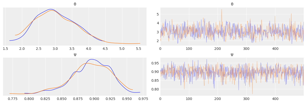
az.summary(mcmc7)
| mean | sd | hdi_3% | hdi_97% | mcse_mean | mcse_sd | ess_bulk | ess_tail | r_hat | |
|---|---|---|---|---|---|---|---|---|---|
| θ | 3.003 | 0.59 | 2.080 | 4.214 | 0.024 | 0.017 | 580.0 | 568.0 | 1.0 |
| ψ | 0.895 | 0.03 | 0.839 | 0.949 | 0.001 | 0.001 | 1062.0 | 689.0 | 1.0 |
Poisson regression and ZIP regression
fish_data = pd.read_csv('../data/fish.csv')
def model(obs=None):
    ψ = numpyro.sample('ψ', dist.Beta(concentration1=1, concentration0=1))
    α = numpyro.sample('α', dist.Normal(loc=0, scale=10))
    β = numpyro.sample('β', dist.Normal(loc=0, scale=10), sample_shape=(2,))

    θ = jnp.exp(α + β[0] * jnp.asarray(fish_data['child']) + β[1] * jnp.asarray(fish_data['camper']))

    yl = numpyro.sample('yl', dist.ZeroInflatedPoisson(gate=ψ, rate=θ), obs=obs)

kernel = NUTS(model)
mcmc8 = MCMC(kernel, num_warmup=500, num_samples=500, num_chains=2, chain_method='sequential')
mcmc8.run(random.PRNGKey(seed), obs=jnp.asarray(fish_data['count']))

az.plot_trace(mcmc8, compact=False, combined=False);
sample: 100%|██████████████████████████| 1000/1000 [00:08<00:00, 121.26it/s, 15 steps of size 3.07e-01. acc. prob=0.94]
sample: 100%|██████████████████████████| 1000/1000 [00:00<00:00, 1955.92it/s, 7 steps of size 3.07e-01. acc. prob=0.92]
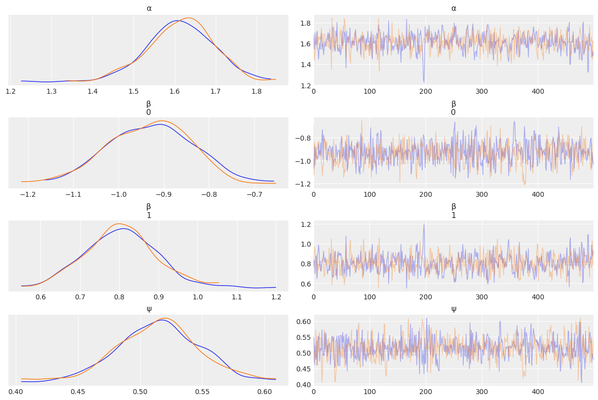
az.summary(mcmc8)
| mean | sd | hdi_3% | hdi_97% | mcse_mean | mcse_sd | ess_bulk | ess_tail | r_hat | |
|---|---|---|---|---|---|---|---|---|---|
| α | 1.613 | 0.083 | 1.462 | 1.769 | 0.003 | 0.002 | 622.0 | 771.0 | 1.0 |
| β[0] | -0.930 | 0.094 | -1.106 | -0.762 | 0.004 | 0.003 | 674.0 | 605.0 | 1.0 |
| β[1] | 0.805 | 0.091 | 0.625 | 0.965 | 0.004 | 0.003 | 623.0 | 539.0 | 1.0 |
| ψ | 0.515 | 0.034 | 0.451 | 0.580 | 0.001 | 0.001 | 714.0 | 487.0 | 1.0 |
children = [0, 1, 2, 3, 4]
fish_count_pred_0 = []
fish_count_pred_1 = []
for n in children:
    without_camper = mcmc8.get_samples()['α'] + mcmc8.get_samples()['β'][:,0] * n
    with_camper = without_camper + mcmc8.get_samples()['β'][:,1]
    fish_count_pred_0.append(jnp.exp(without_camper))
    fish_count_pred_1.append(jnp.exp(with_camper))


plt.plot(children, fish_count_pred_0, 'C0.', alpha=0.01)
plt.plot(children, fish_count_pred_1, 'C1.', alpha=0.01)

plt.xticks(children);
plt.xlabel('Number of children')
plt.ylabel('Fish caught')
plt.plot([], 'C0o', label='without camper')
plt.plot([], 'C1o', label='with camper')
plt.legend()
<matplotlib.legend.Legend at 0x134b48df0>

Robust logistic regression
iris = sns.load_dataset("iris")
df = iris.query("species == ('setosa', 'versicolor')")
y_0 = pd.Categorical(df['species']).codes
x_n = 'sepal_length'
x_0 = df[x_n].values
y_0 = jnp.concatenate((y_0, jnp.ones(6, dtype=int)))
x_0 = jnp.concatenate((x_0, jnp.array([4.2, 4.5, 4.0, 4.3, 4.2, 4.4])))
x_c = x_0 - x_0.mean()
plt.plot(x_c, y_0, 'o', color='k');

def model(obs=None):

    α = numpyro.sample('α', dist.Normal(loc=0, scale=10))
    β = numpyro.sample('β', dist.Normal(loc=0, scale=10))

    μ = α + x_c *  β
    θ = numpyro.deterministic('θ', jnn.sigmoid(μ))
    bd = numpyro.deterministic('bd', -α/β)

    π = numpyro.sample('π', dist.Beta(concentration1=1., concentration0=1.))
    p = π * 0.5 + (1 - π) * θ

    yl = numpyro.sample('yl', dist.Bernoulli(probs=p), obs=obs)

kernel = NUTS(model)
mcmc9 = MCMC(kernel, num_warmup=500, num_samples=500, num_chains=2, chain_method='sequential')
mcmc9.run(random.PRNGKey(seed), obs=y_0)
sample: 100%|███████████████████████████| 1000/1000 [00:05<00:00, 197.06it/s, 7 steps of size 5.13e-01. acc. prob=0.89]
sample: 100%|██████████████████████████| 1000/1000 [00:00<00:00, 2268.58it/s, 7 steps of size 5.08e-01. acc. prob=0.90]
az.plot_trace(mcmc9, varnames, compact=False, combined=False);

varnames = ['α', 'β', 'bd']
az.summary(mcmc9, varnames)
| mean | sd | hdi_3% | hdi_97% | mcse_mean | mcse_sd | ess_bulk | ess_tail | r_hat | |
|---|---|---|---|---|---|---|---|---|---|
| α | -0.803 | 0.877 | -2.483 | 0.814 | 0.036 | 0.026 | 609.0 | 584.0 | 1.0 |
| β | 16.157 | 6.057 | 5.312 | 26.757 | 0.282 | 0.202 | 479.0 | 647.0 | 1.0 |
| bd | 0.047 | 0.053 | -0.061 | 0.143 | 0.002 | 0.001 | 755.0 | 632.0 | 1.0 |
theta = mcmc9.get_samples()['θ'].mean(axis=0)
idx = jnp.argsort(x_c)
plt.plot(x_c[idx], theta[idx], color='C2', lw=3);
plt.vlines(mcmc9.get_samples()['bd'].mean(), 0, 1, color='k')
bd_hdi = az.hdi(mcmc9.get_samples()['bd'].copy())

plt.fill_betweenx([0, 1], bd_hdi[0], bd_hdi[1], color='k', alpha=0.5)

plt.scatter(x_c, dist.Normal(y_0, 0.02).sample(random.PRNGKey(1)), marker='.', color=[f'C{x}' for x in y_0])
theta_hdi = az.hdi(mcmc9.get_samples()['θ'].copy())[idx]
plt.fill_between(x_c[idx], theta_hdi[:,0], theta_hdi[:,1], color='C2', alpha=0.5)

plt.xlabel(x_n)
plt.ylabel('θ', rotation=0)
# use original scale for xticks
locs, _ = plt.xticks()
plt.xticks(locs, jnp.round(locs + x_0.mean(), 1))
FutureWarning: hdi currently interprets 2d data as (draw, shape) but this will change in a future release to (chain, draw) for coherence with other functions
([<matplotlib.axis.XTick at 0x13680e4f0>,
  <matplotlib.axis.XTick at 0x13680e4c0>,
  <matplotlib.axis.XTick at 0x1367e5d90>,
  <matplotlib.axis.XTick at 0x136862eb0>,
  <matplotlib.axis.XTick at 0x136855e20>,
  <matplotlib.axis.XTick at 0x136872940>,
  <matplotlib.axis.XTick at 0x13687e0a0>,
  <matplotlib.axis.XTick at 0x13687e5b0>,
  <matplotlib.axis.XTick at 0x136862e20>],
 [Text(-2.0, 0, '3.4'),
  Text(-1.5, 0, '3.9'),
  Text(-1.0, 0, '4.4'),
  Text(-0.5, 0, '4.9'),
  Text(0.0, 0, '5.4'),
  Text(0.5, 0, '5.9'),
  Text(1.0, 0, '6.4'),
  Text(1.5, 0, '6.9'),
  Text(2.0, 0, '7.4')])
