.ipynb .pdf

repository open issue suggest edit

Binder Colab

Contents

Chapter 3. Modeling with Linear Regressions

import os
import warnings

import arviz as az
import matplotlib.pyplot as plt
import pandas as pd
from scipy.interpolate import BSpline
from scipy.stats import gaussian_kde

import jax.numpy as jnp
from jax import random, vmap, local_device_count, pmap

import numpyro
import numpyro.distributions as dist
import numpyro.optim as optim

from numpyro.infer import MCMC, NUTS, HMC, Predictive
from numpyro.diagnostics import hpdi, print_summary
from numpyro.infer import Predictive, SVI, Trace_ELBO, init_to_value
from numpyro.infer.autoguide import AutoLaplaceApproximation


seed=1234

if "SVG" in os.environ:
    %config InlineBackend.figure_formats = ["svg"]
warnings.formatwarning = lambda message, category, *args, **kwargs: "{}: {}\n".format(
    category.__name__, message
)
az.style.use("arviz-darkgrid")
numpyro.set_platform("cpu") # or "gpu", "tpu" depending on system
numpyro.set_host_device_count(local_device_count())

# import pymc3 as pm
# import numpy as np
# import pandas as pd
# from theano import shared
# import scipy.stats as stats
# import matplotlib.pyplot as plt
# import arviz as az

# az.style.use('arviz-darkgrid')

Simple linear regression

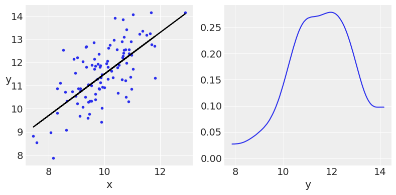
N = 100
alpha_real = 2.5
beta_real = 0.9

eps_real = dist.Normal(loc=0, scale=1).sample(random.PRNGKey(0), (N,))

x = dist.Normal(loc=10, scale=1.).sample(random.PRNGKey(1), (N,)) # Same seed produces perfect line
y_real = alpha_real + beta_real * x
y = y_real + eps_real

# we can center the data
# x = x - x.mean()
# or standardize the data
# x = (x - x.mean())/x.std()
# y = (y - y.mean())/y.std()

_, ax = plt.subplots(1, 2, figsize=(8, 4))
ax[0].plot(x, y, 'C0.')
ax[0].set_xlabel('x')
ax[0].set_ylabel('y', rotation=0)
ax[0].plot(x, y_real, 'k')

az.plot_kde(y, ax=ax[1])
ax[1].set_xlabel('y')
plt.tight_layout()

UserWarning: This figure was using constrained_layout, but that is incompatible with subplots_adjust and/or tight_layout; disabling constrained_layout.

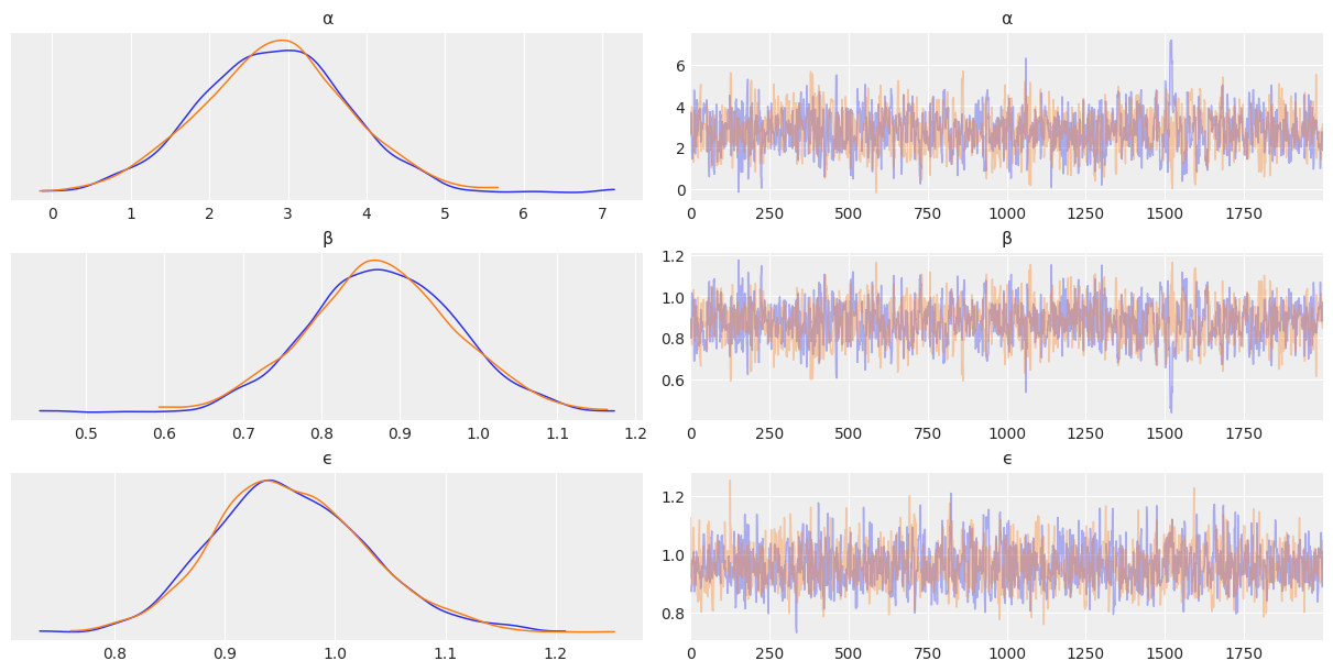
def model(obs=None):
    α = numpyro.sample('α', dist.Normal(loc=0, scale=10))
    β = numpyro.sample('β', dist.Normal(loc=0, scale=1))
    ϵ = numpyro.sample('ϵ', dist.HalfCauchy(scale=5))
    
    μ = numpyro.deterministic('μ', α + β * x)
    
    y_pred = numpyro.sample('y_pred', dist.Normal(loc=μ, scale=ϵ), obs=obs, sample_shape=(len(y),))
        
kernel = NUTS(model)
mcmc = MCMC(kernel, num_warmup=1000, num_samples=2000, num_chains=2)
mcmc.run(random.PRNGKey(seed), obs=y)

UserWarning: There are not enough devices to run parallel chains: expected 2 but got 1. Chains will be drawn sequentially. If you are running MCMC in CPU, consider using `numpyro.set_host_device_count(2)` at the beginning of your program. You can double-check how many devices are available in your system using `jax.local_device_count()`.
sample: 100%|███████████████████████████████████████████| 3000/3000 [00:06<00:00, 471.97it/s, 63 steps of size 5.89e-02. acc. prob=0.94]
sample: 100%|██████████████████████████████████████████| 3000/3000 [00:00<00:00, 3828.37it/s, 11 steps of size 6.59e-02. acc. prob=0.94]

az.plot_trace(mcmc, var_names=['α', 'β', 'ϵ'], compact=False)

array([[<AxesSubplot:title={'center':'α'}>,
        <AxesSubplot:title={'center':'α'}>],
       [<AxesSubplot:title={'center':'β'}>,
        <AxesSubplot:title={'center':'β'}>],
       [<AxesSubplot:title={'center':'ϵ'}>,
        <AxesSubplot:title={'center':'ϵ'}>]], dtype=object)

Modyfing the data before running the models

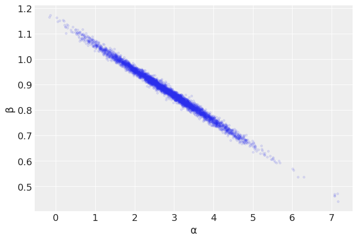
az.plot_pair(mcmc, var_names=['α', 'β'], scatter_kwargs={'alpha': 0.1})  # UserWarning: plot_kwargs will be deprecated. Please use scatter_kwargs, kde_kwargs and/or hexbin_kwargs

<AxesSubplot:xlabel='α', ylabel='β'>

interpreting the posterior

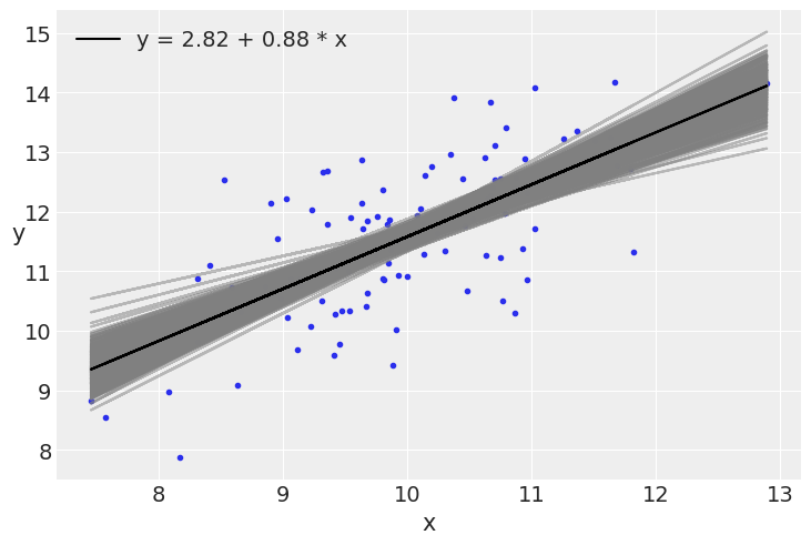
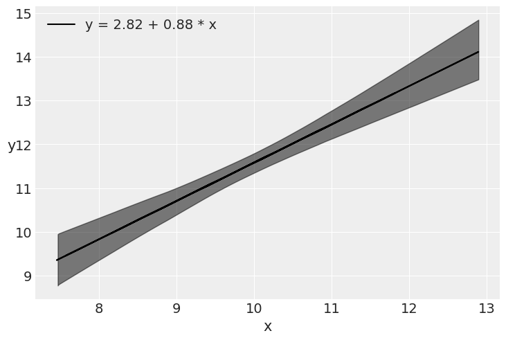
plt.plot(x, y, 'C0.')

alpha_m = mcmc.get_samples()['α'].mean()
beta_m = mcmc.get_samples()['β'].mean()

draws = range(0, len(mcmc.get_samples()['α']), 10)
plt.plot(x, mcmc.get_samples()['α'][jnp.array(draws)] + mcmc.get_samples()['β'][jnp.array(draws)]  # https://github.com/google/jax/issues/4564
         * x[:, jnp.newaxis], c='gray', alpha=0.5)

plt.plot(x, alpha_m + beta_m * x, c='k',
         label=f'y = {alpha_m:.2f} + {beta_m:.2f} * x')

plt.xlabel('x')
plt.ylabel('y', rotation=0)
plt.legend()

<matplotlib.legend.Legend at 0x7fb474c54520>

plt.plot(x, alpha_m + beta_m * x, c='k',
         label=f'y = {alpha_m:.2f} + {beta_m:.2f} * x')

sig = az.plot_hdi(x, mcmc.get_samples()['μ'], hdi_prob=0.98, color='k')

plt.xlabel('x')
plt.ylabel('y', rotation=0)
plt.legend()

FutureWarning: hdi currently interprets 2d data as (draw, shape) but this will change in a future release to (chain, draw) for coherence with other functions

<matplotlib.legend.Legend at 0x7fb472fa1ca0>

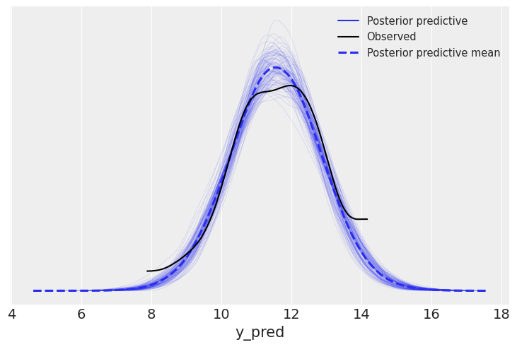
pred = Predictive(model=mcmc.sampler.model, posterior_samples=mcmc.get_samples(), return_sites=['y_pred'])
ppc = pred(random.PRNGKey(seed))

ppc['y_pred'].shape

(4000, 100, 100)

ppc['y_pred'] = ppc['y_pred'][:100]
ppc['y_pred'].shape

(100, 100, 100)

samples = az.from_numpyro(mcmc, posterior_predictive=ppc)
az.plot_ppc(samples, mean=True, observed=True, alpha=0.1)

WARNING:arviz.data.io_numpyro:posterior predictive shape not compatible with number of chains and draws. This can mean that some draws or even whole chains are not represented.

<AxesSubplot:xlabel='y_pred'>

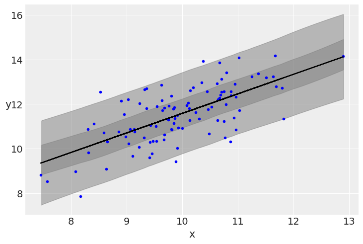
plt.plot(x, y, 'b.')
plt.plot(x, alpha_m + beta_m * x, c='k',
         label=f'y = {alpha_m:.2f} + {beta_m:.2f} * x')

az.plot_hdi(x, ppc['y_pred'], hdi_prob=0.5, color='gray')
az.plot_hdi(x, ppc['y_pred'], color='gray')

plt.xlabel('x')
plt.ylabel('y', rotation=0)

Text(0, 0.5, 'y')

az.r2_score(y, ppc['y_pred'])

r2        0.44905096
r2_std    0.03545001
dtype: object

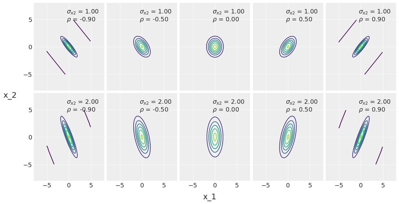
The multivariate normal distribution

Actually the bivariate

sigma_x1 = 1
sigmas_x2 = [1, 2]
rhos = [-0.90, -0.5, 0, 0.5, 0.90]

k, l = jnp.mgrid[-5:5:.1, -5:5:.1]
pos = jnp.empty(k.shape + (2,))
# pos[:, :, 0] = k
# pos[:, :, 1] = l
pos = pos.at[:, :, 0].set(k)
pos = pos.at[:, :, 1].set(l)


f, ax = plt.subplots(len(sigmas_x2), len(rhos),
                     sharex=True, sharey=True, figsize=(12, 6),
                     constrained_layout=True)
for i in range(2):
    for j in range(5):
        sigma_x2 = sigmas_x2[i]
        rho = rhos[j]
        cov = [[sigma_x1**2, sigma_x1*sigma_x2*rho],
               [sigma_x1*sigma_x2*rho, sigma_x2**2]]
        
        rv = dist.MultivariateNormal(jnp.array([0,0]), covariance_matrix=cov)

        ax[i, j].contour(k, l, jnp.exp(rv.log_prob(pos)), levels=6)
        ax[i, j].set_xlim(-8, 8)
        ax[i, j].set_ylim(-8, 8)
        ax[i, j].set_yticks([-5, 0, 5])
        ax[i, j].plot(0, 0, label=f'$\\sigma_{{x2}}$ = {sigma_x2:3.2f}\n$\\rho$ = {rho:3.2f}', alpha=0)
        ax[i, j].legend()
f.text(0.5, -0.05, 'x_1', ha='center', fontsize=18)
f.text(-0.05, 0.5, 'x_2', va='center', fontsize=18, rotation=0)

Text(-0.05, 0.5, 'x_2')

data = jnp.stack((x, y)).T

def model(obs=None):
    
    μ = numpyro.sample('μ', dist.Normal(loc=data.mean(0), scale=10))
    
    σ_1 = numpyro.sample('σ_1', dist.HalfNormal(scale=10))
    σ_2 = numpyro.sample('σ_2', dist.HalfNormal(scale=10))
    ρ = numpyro.sample('ρ', dist.Uniform(low=-1., high=1.))
    
    r2 = numpyro.deterministic('r2', ρ**2)
    
    cov = jnp.stack((jnp.array([σ_1**2, σ_1*σ_2*ρ]),
                    jnp.array([σ_1*σ_2*ρ, σ_2**2])))
    
    y_pred = numpyro.sample('y_pred', dist.MultivariateNormal(loc=μ, covariance_matrix=cov), obs=obs)
    
kernel = NUTS(model)
mcmc2 = MCMC(kernel, num_warmup=1000, num_samples=1000, num_chains=2)
mcmc2.run(random.PRNGKey(seed), obs=data)

UserWarning: There are not enough devices to run parallel chains: expected 2 but got 1. Chains will be drawn sequentially. If you are running MCMC in CPU, consider using `numpyro.set_host_device_count(2)` at the beginning of your program. You can double-check how many devices are available in your system using `jax.local_device_count()`.
sample: 100%|████████████████████████████████████████████| 2000/2000 [00:03<00:00, 532.16it/s, 7 steps of size 4.81e-01. acc. prob=0.92]
sample: 100%|███████████████████████████████████████████| 2000/2000 [00:00<00:00, 4882.91it/s, 3 steps of size 6.17e-01. acc. prob=0.86]

az.plot_trace(mcmc2, var_names=['r2'], compact=False)

array([[<AxesSubplot:title={'center':'r2'}>,
        <AxesSubplot:title={'center':'r2'}>]], dtype=object)

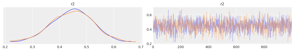
az.summary(mcmc2, var_names=['r2'])

	mean	sd	hdi_3%	hdi_97%	mcse_mean	mcse_sd	ess_bulk	ess_tail	r_hat
r2	0.447	0.075	0.314	0.596	0.002	0.001	1432.0	1332.0	1.0

Robust linear regression

ans = pd.read_csv('../data/anscombe.csv')
x_3 = ans[ans.group == 'III']['x'].values
y_3 = ans[ans.group == 'III']['y'].values
x_3 = x_3 - x_3.mean()

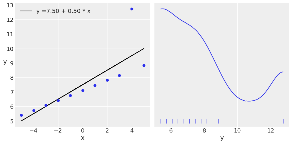
_, ax = plt.subplots(1, 2, figsize=(10, 5))
beta_c, alpha_c = jnp.polyfit(x_3, y_3, deg=1) # equivulant to stats.linregress(x_3, y_3)[:2]
ax[0].plot(x_3, (alpha_c + beta_c * x_3), 'k',
           label=f'y ={alpha_c:.2f} + {beta_c:.2f} * x')
ax[0].plot(x_3, y_3, 'C0o')
ax[0].set_xlabel('x')
ax[0].set_ylabel('y', rotation=0)
ax[0].legend(loc=0)
az.plot_kde(y_3, ax=ax[1], rug=True)
ax[1].set_xlabel('y')
ax[1].set_yticks([])
plt.tight_layout()

UserWarning: This figure was using constrained_layout, but that is incompatible with subplots_adjust and/or tight_layout; disabling constrained_layout.

def model(obs=None):
    α = numpyro.sample('α', dist.Normal(loc=y_3.mean(), scale=1))
    β = numpyro.sample('β', dist.Normal(loc=0, scale=1))
    ϵ = numpyro.sample('ϵ', dist.HalfNormal(scale=5))
    ν_ = numpyro.sample('ν_', dist.Exponential(rate=1/29))
    ν = numpyro.deterministic('ν', ν_ + 1)

    y_pred = numpyro.sample('y_pred', dist.StudentT(df=ν, loc=α + β * x_3, scale=ϵ), obs=obs)
    
kernel = NUTS(model)
mcmc3 = MCMC(kernel, num_warmup=1000, num_samples=1000, num_chains=4)
mcmc3.run(random.PRNGKey(seed), obs=y_3)

UserWarning: There are not enough devices to run parallel chains: expected 4 but got 1. Chains will be drawn sequentially. If you are running MCMC in CPU, consider using `numpyro.set_host_device_count(4)` at the beginning of your program. You can double-check how many devices are available in your system using `jax.local_device_count()`.
sample: 100%|███████████████████████████████████████████| 2000/2000 [00:03<00:00, 569.98it/s, 15 steps of size 9.41e-02. acc. prob=0.84]
sample: 100%|██████████████████████████████████████████| 2000/2000 [00:00<00:00, 4779.28it/s, 27 steps of size 1.24e-01. acc. prob=0.72]
sample: 100%|██████████████████████████████████████████| 2000/2000 [00:00<00:00, 4806.93it/s, 23 steps of size 1.20e-01. acc. prob=0.74]
sample: 100%|██████████████████████████████████████████| 2000/2000 [00:00<00:00, 4882.93it/s, 15 steps of size 1.06e-01. acc. prob=0.81]

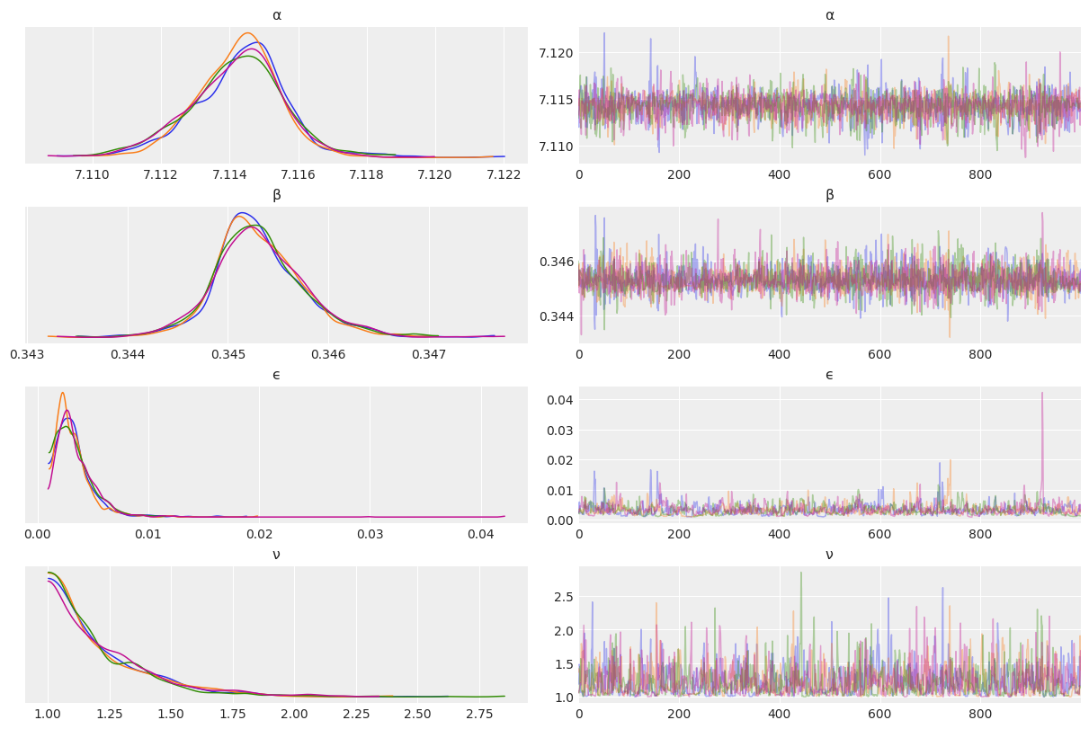
varnames = ['α', 'β', 'ϵ', 'ν']
az.plot_trace(mcmc3, var_names=varnames, compact=False);

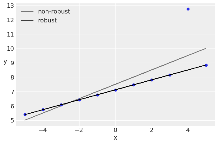
beta_c, alpha_c = jnp.polyfit(x_3, y_3, deg=1) 

plt.plot(x_3, (alpha_c + beta_c * x_3), 'k', label='non-robust', alpha=0.5)
plt.plot(x_3, y_3, 'C0o')
alpha_m = jnp.mean(mcmc3.get_samples()['α'])
beta_m = jnp.mean(mcmc3.get_samples()['β'])
plt.plot(x_3, alpha_m + beta_m * x_3, c='k', label='robust')

plt.xlabel('x')
plt.ylabel('y', rotation=0)
plt.legend(loc=2)
plt.tight_layout()

UserWarning: This figure was using constrained_layout, but that is incompatible with subplots_adjust and/or tight_layout; disabling constrained_layout.

az.summary(mcmc3, var_names=varnames)

	mean	sd	hdi_3%	hdi_97%	mcse_mean	mcse_sd	ess_bulk	ess_tail	r_hat
α	7.114	0.001	7.112	7.117	0.000	0.000	3155.0	2179.0	1.00
β	0.345	0.000	0.345	0.346	0.000	0.000	3861.0	2209.0	1.00
ϵ	0.003	0.002	0.001	0.006	0.000	0.000	402.0	327.0	1.01
ν	1.219	0.214	1.000	1.604	0.006	0.004	906.0	847.0	1.00

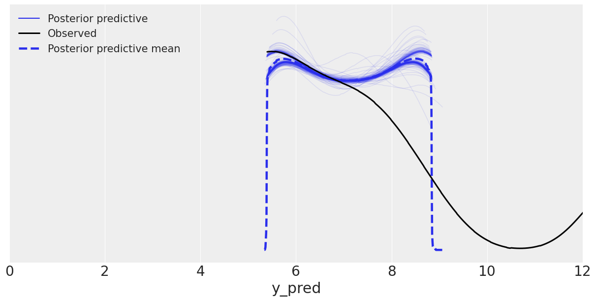
pred = Predictive(model=mcmc3.sampler.model, posterior_samples=mcmc3.get_samples(), return_sites=['y_pred'])
ppc = pred(random.PRNGKey(seed))

ppc['y_pred'] = ppc['y_pred'][:200]
ppc['y_pred'].shape

(200, 11)

data_ppc = az.from_numpyro(mcmc3, posterior_predictive=ppc)
az.plot_ppc(data_ppc, figsize=(12, 6), mean=True, alpha=0.1, color='C0')
plt.xlim(0, 12)

WARNING:arviz.data.io_numpyro:posterior predictive shape not compatible with number of chains and draws. This can mean that some draws or even whole chains are not represented.

(0.0, 12.0)

Hierarchical linear regression

N = 20
M = 8
idx = jnp.repeat(jnp.arange(M-1), N)
idx = jnp.append(idx, 7)

# alpha_real = numpyro.sample('alpha_real', dist.Normal(loc=2.5, scale=0.5), sample_shape=(M,)) 
alpha_real = dist.Normal(loc=2.5, scale=0.5).sample(random.PRNGKey(seed), (M,))
beta_real = dist.Beta(concentration1=6, concentration0=1).sample(random.PRNGKey(seed), (M,))
eps_real = dist.Normal(loc=0, scale=0.5).sample(random.PRNGKey(seed+1), (len(idx),))
                                                
y_m = jnp.zeros(len(idx))
x_m = dist.Normal(loc=10, scale=1.).sample(random.PRNGKey(seed), (len(idx),))
                                           
y_m = alpha_real[idx] + beta_real[idx] * x_m + eps_real

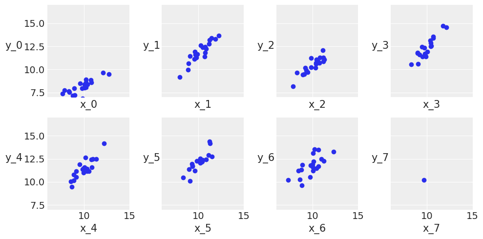
_, ax = plt.subplots(2, 4, figsize=(10, 5), sharex=True, sharey=True)
ax = list(ax.flat) # np.ravel(ax)
j, k = 0, N
for i in range(M):
    ax[i].scatter(x_m[j:k], y_m[j:k])
    ax[i].set_xlabel(f'x_{i}')
    ax[i].set_ylabel(f'y_{i}', rotation=0, labelpad=15)
    ax[i].set_xlim(6, 15)
    ax[i].set_ylim(7, 17)
    j += N
    k += N
plt.tight_layout()

UserWarning: This figure was using constrained_layout, but that is incompatible with subplots_adjust and/or tight_layout; disabling constrained_layout.

x_centered = x_m - x_m.mean()

def model(obs=None):
    with numpyro.handlers.seed(rng_seed=seed):
        α_tmp = numpyro.sample("α_tmp", dist.Normal(loc=0, scale=10).expand([M]))
        β = numpyro.sample("β", dist.Normal(loc=0, scale=10).expand([M]))
    
    ϵ = numpyro.sample('ϵ', dist.HalfCauchy(scale=5))
    ν = numpyro.sample('ν', dist.Exponential(rate=1/30))
    
    y_pred = numpyro.sample('y_pred', dist.StudentT(df=ν, loc=α_tmp[idx] + β[idx] * x_centered, scale=ϵ), obs=obs)
    
    α = numpyro.deterministic('α', α_tmp - β * x_m.mean())
    
kernel = NUTS(model)
mcmc4 = MCMC(kernel, num_warmup=1000, num_samples=1000, num_chains=4, chain_method='sequential')
mcmc4.run(random.PRNGKey(seed), obs=y_m)

sample: 100%|███████████████████████████████████████████| 2000/2000 [00:04<00:00, 425.80it/s, 31 steps of size 1.15e-01. acc. prob=0.93]
sample: 100%|██████████████████████████████████████████| 2000/2000 [00:00<00:00, 3402.84it/s, 31 steps of size 1.13e-01. acc. prob=0.92]
sample: 100%|██████████████████████████████████████████| 2000/2000 [00:00<00:00, 4030.06it/s, 31 steps of size 1.20e-01. acc. prob=0.92]
sample: 100%|██████████████████████████████████████████| 2000/2000 [00:00<00:00, 3526.99it/s, 63 steps of size 8.52e-02. acc. prob=0.96]

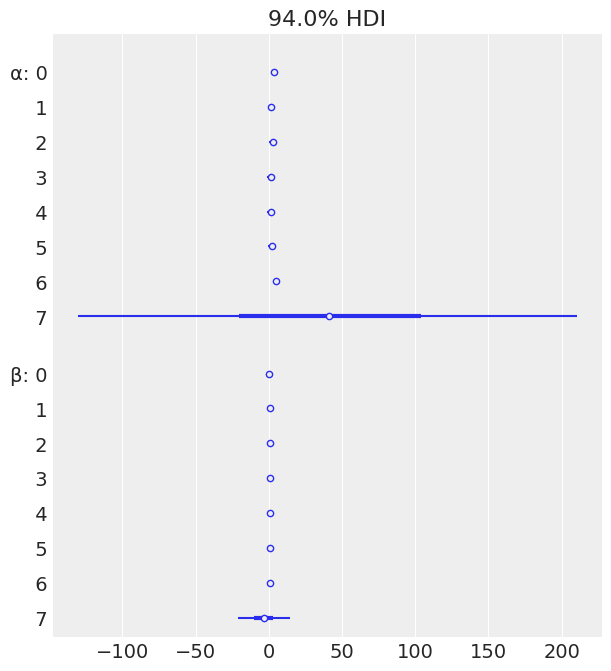
az.plot_forest(mcmc4, var_names=['α', 'β'], combined=True)

array([<AxesSubplot:title={'center':'94.0% HDI'}>], dtype=object)

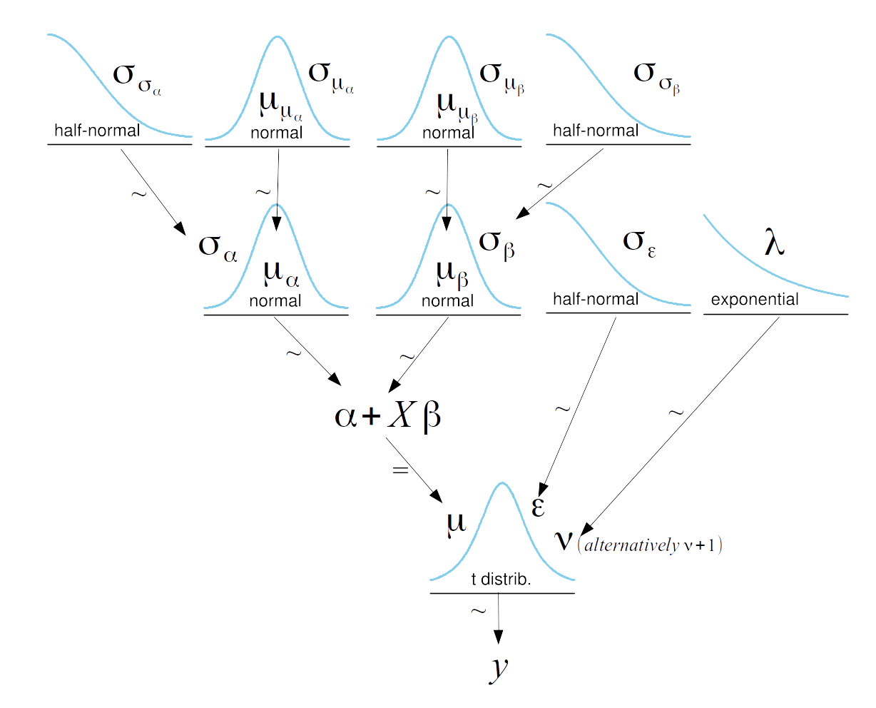
def model(obs=None):
    # Hyper-priors
    α_μ_tmp = numpyro.sample('α_μ_tmp', dist.Normal(loc=0, scale=10))
    α_σ_tmp = numpyro.sample('α_σ_tmp', dist.HalfNormal(scale=10))
    β_μ = numpyro.sample('β_μ', dist.Normal(loc=0, scale=10))
    β_σ = numpyro.sample('β_σ', dist.HalfNormal(scale=10))
    
    # Priors
    with numpyro.handlers.seed(rng_seed=seed):
        α_tmp = numpyro.sample("α_tmp", dist.Normal(loc=α_μ_tmp, scale=α_σ_tmp).expand([M]))
        β = numpyro.sample("β", dist.Normal(loc=β_μ, scale=β_σ).expand([M]))
    ϵ = numpyro.sample('ϵ', dist.HalfCauchy(scale=5))
    ν = numpyro.sample('ν', dist.Exponential(rate=1/30))
    
    y_pred = numpyro.sample('y_pred', dist.StudentT(df=ν, loc=α_tmp[idx] + β[idx] * x_centered, scale=ϵ), obs=obs)
    
    α = numpyro.deterministic('α', α_tmp - β * x_m.mean())
    α_μ = numpyro.deterministic('α_μ', α_μ_tmp - β_μ * x_m.mean())
    α_σ = numpyro.deterministic('α_sd', α_σ_tmp - β_μ * x_m.mean())
    
kernel = NUTS(model)
mcmc5 = MCMC(kernel, num_warmup=1000, num_samples=1000, num_chains=4, chain_method='sequential')
mcmc5.run(random.PRNGKey(seed), obs=y_m)

sample: 100%|████████████████████████████████████████████| 2000/2000 [00:07<00:00, 269.98it/s, 7 steps of size 4.08e-01. acc. prob=0.88]
sample: 100%|██████████████████████████████████████████| 2000/2000 [00:00<00:00, 3869.46it/s, 15 steps of size 3.79e-01. acc. prob=0.91]
sample: 100%|███████████████████████████████████████████| 2000/2000 [00:00<00:00, 3576.93it/s, 7 steps of size 3.63e-01. acc. prob=0.88]
sample: 100%|██████████████████████████████████████████| 2000/2000 [00:00<00:00, 3715.94it/s, 15 steps of size 4.17e-01. acc. prob=0.83]

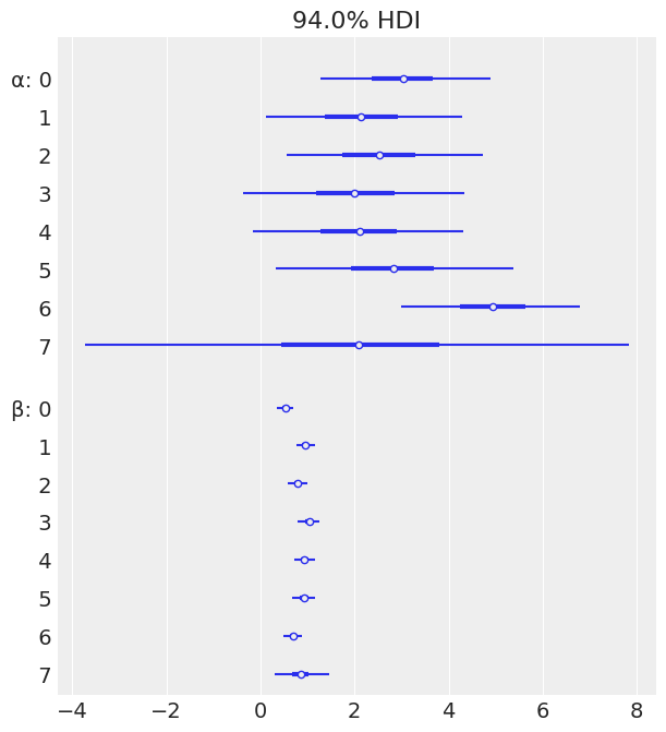
az.plot_forest(mcmc5, var_names=['α', 'β'], combined=True)

array([<AxesSubplot:title={'center':'94.0% HDI'}>], dtype=object)

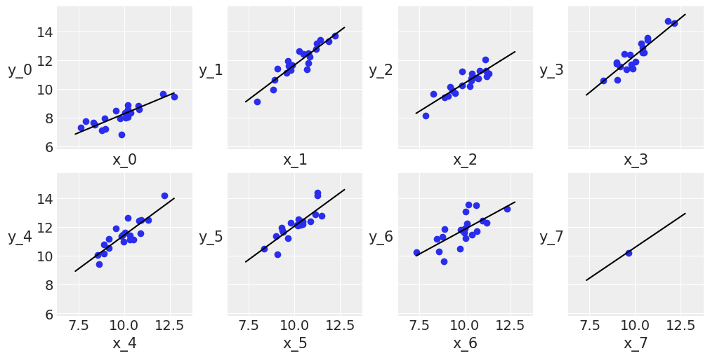
_, ax = plt.subplots(2, 4, figsize=(10, 5), sharex=True, sharey=True, constrained_layout=True)
ax = list(ax.flat) # np.ravel(ax)

j, k = 0, N
x_range = jnp.linspace(x_m.min(), x_m.max(), 10)

for i in range(M):

    ax[i].scatter(x_m[j:k], y_m[j:k])
    ax[i].set_xlabel(f'x_{i}')
    ax[i].set_ylabel(f'y_{i}', labelpad=17, rotation=0)
    
    alpha_m = mcmc5.get_samples()['α'][:, i].mean()
    beta_m = mcmc5.get_samples()['β'][:, i].mean()
    
    ax[i].plot(x_range, alpha_m + beta_m * x_range, c='k', label=f'y = {alpha_m:.2f} + {beta_m:.2f} * x')
    
    plt.xlim(x_m.min()-1, x_m.max()+1)
    plt.ylim(y_m.min()-1, y_m.max()+1)
    
    j += N
    k += N

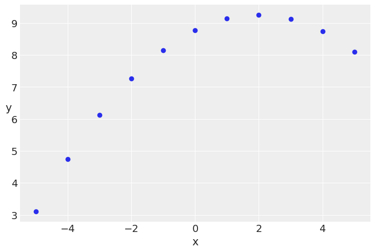
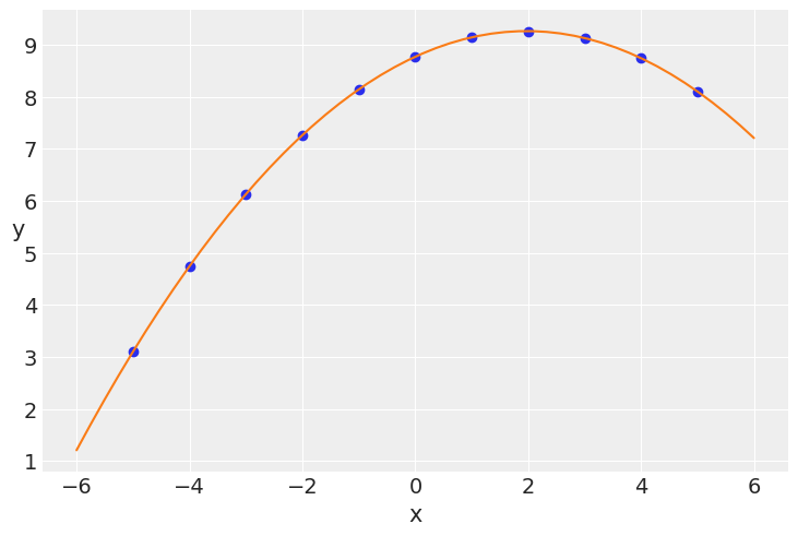
Polynomial regression

x_2 = ans[ans.group == 'II']['x'].values
y_2 = ans[ans.group == 'II']['y'].values
x_2 = x_2 - x_2.mean()

plt.scatter(x_2, y_2)
plt.xlabel('x')
plt.ylabel('y', rotation=0)

Text(0, 0.5, 'y')

def model(obs=None):
    
    α = numpyro.sample("α", dist.Normal(loc=y_2.mean(), scale=1))
    β1 = numpyro.sample("β1", dist.Normal(loc=0, scale=1))
    β2 = numpyro.sample("β2", dist.Normal(loc=0, scale=1))
    ϵ = numpyro.sample('ϵ', dist.HalfCauchy(scale=5))
                        
    mu = numpyro.deterministic('mu', α + β1 * x_2 + β2 * x_2**2)
                            
    y_pred = numpyro.sample('y_pred', dist.Normal(loc=mu, scale=ϵ), obs=obs)
    

kernel = NUTS(model)
mcmc6 = MCMC(kernel, num_warmup=1000, num_samples=1000, num_chains=4, chain_method='sequential')
mcmc6.run(random.PRNGKey(seed), obs=y_2)

sample: 100%|███████████████████████████████████████████| 2000/2000 [00:03<00:00, 550.88it/s, 19 steps of size 1.23e-02. acc. prob=0.94]
sample: 100%|██████████████████████████████████████████| 2000/2000 [00:00<00:00, 4792.22it/s, 83 steps of size 1.43e-02. acc. prob=0.90]
sample: 100%|██████████████████████████████████████████| 2000/2000 [00:00<00:00, 4870.41it/s, 79 steps of size 1.28e-02. acc. prob=0.93]
sample: 100%|██████████████████████████████████████████| 2000/2000 [00:00<00:00, 4296.65it/s, 35 steps of size 1.52e-02. acc. prob=0.88]

az.plot_trace(mcmc6, compact=False)

array([[<AxesSubplot:title={'center':'mu\n0'}>,
        <AxesSubplot:title={'center':'mu\n0'}>],
       [<AxesSubplot:title={'center':'mu\n1'}>,
        <AxesSubplot:title={'center':'mu\n1'}>],
       [<AxesSubplot:title={'center':'mu\n2'}>,
        <AxesSubplot:title={'center':'mu\n2'}>],
       [<AxesSubplot:title={'center':'mu\n3'}>,
        <AxesSubplot:title={'center':'mu\n3'}>],
       [<AxesSubplot:title={'center':'mu\n4'}>,
        <AxesSubplot:title={'center':'mu\n4'}>],
       [<AxesSubplot:title={'center':'mu\n5'}>,
        <AxesSubplot:title={'center':'mu\n5'}>],
       [<AxesSubplot:title={'center':'mu\n6'}>,
        <AxesSubplot:title={'center':'mu\n6'}>],
       [<AxesSubplot:title={'center':'mu\n7'}>,
        <AxesSubplot:title={'center':'mu\n7'}>],
       [<AxesSubplot:title={'center':'mu\n8'}>,
        <AxesSubplot:title={'center':'mu\n8'}>],
       [<AxesSubplot:title={'center':'mu\n9'}>,
        <AxesSubplot:title={'center':'mu\n9'}>],
       [<AxesSubplot:title={'center':'mu\n10'}>,
        <AxesSubplot:title={'center':'mu\n10'}>],
       [<AxesSubplot:title={'center':'α'}>,
        <AxesSubplot:title={'center':'α'}>],
       [<AxesSubplot:title={'center':'β1'}>,
        <AxesSubplot:title={'center':'β1'}>],
       [<AxesSubplot:title={'center':'β2'}>,
        <AxesSubplot:title={'center':'β2'}>],
       [<AxesSubplot:title={'center':'ϵ'}>,
        <AxesSubplot:title={'center':'ϵ'}>]], dtype=object)

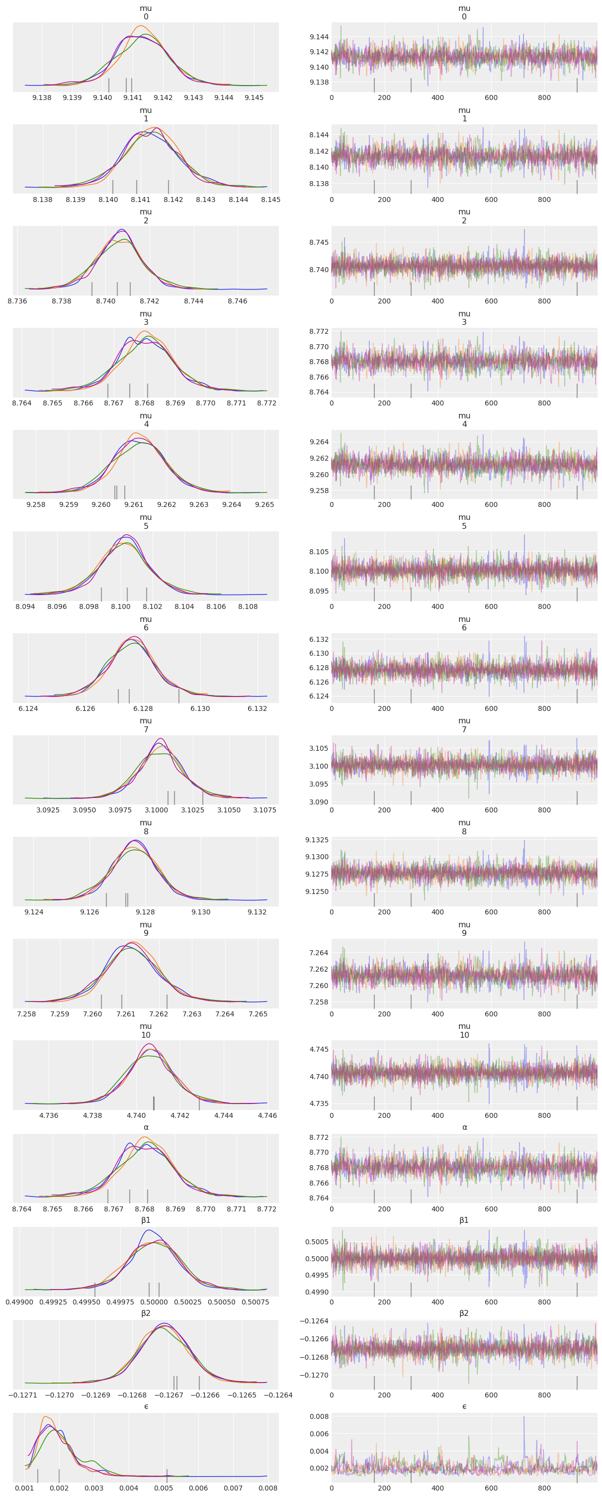
az.summary(mcmc6)

	mean	sd	hdi_3%	hdi_97%	mcse_mean	mcse_sd	ess_bulk	ess_tail	r_hat
mu[0]	9.141	0.001	9.140	9.143	0.0	0.0	1875.0	1538.0	1.00
mu[1]	8.141	0.001	8.140	8.143	0.0	0.0	1795.0	1561.0	1.00
mu[2]	8.741	0.001	8.739	8.743	0.0	0.0	4162.0	2394.0	1.00
mu[3]	8.768	0.001	8.766	8.770	0.0	0.0	1779.0	1578.0	1.00
mu[4]	9.261	0.001	9.260	9.263	0.0	0.0	2218.0	1754.0	1.00
mu[5]	8.100	0.002	8.097	8.103	0.0	0.0	4036.0	2469.0	1.00
mu[6]	6.128	0.001	6.126	6.129	0.0	0.0	2860.0	2225.0	1.00
mu[7]	3.100	0.002	3.097	3.103	0.0	0.0	3767.0	2500.0	1.00
mu[8]	9.128	0.001	9.126	9.129	0.0	0.0	3289.0	2529.0	1.00
mu[9]	7.261	0.001	7.260	7.263	0.0	0.0	2014.0	1849.0	1.00
mu[10]	4.741	0.001	4.739	4.743	0.0	0.0	3828.0	2365.0	1.00
α	8.768	0.001	8.766	8.770	0.0	0.0	1779.0	1578.0	1.00
β1	0.500	0.000	0.500	0.500	0.0	0.0	3816.0	1826.0	1.01
β2	-0.127	0.000	-0.127	-0.127	0.0	0.0	2497.0	2168.0	1.00
ϵ	0.002	0.001	0.001	0.003	0.0	0.0	359.0	735.0	1.02

x_p = jnp.linspace(-6, 6)
y_p = mcmc6.get_samples()['α'].mean() + mcmc6.get_samples()['β1'].mean() * \
    x_p + mcmc6.get_samples()['β2'].mean() * x_p**2
plt.scatter(x_2, y_2)
plt.xlabel('x')
plt.ylabel('y', rotation=0)
plt.plot(x_p, y_p, c='C1')

[<matplotlib.lines.Line2D at 0x7fb442e52dc0>]

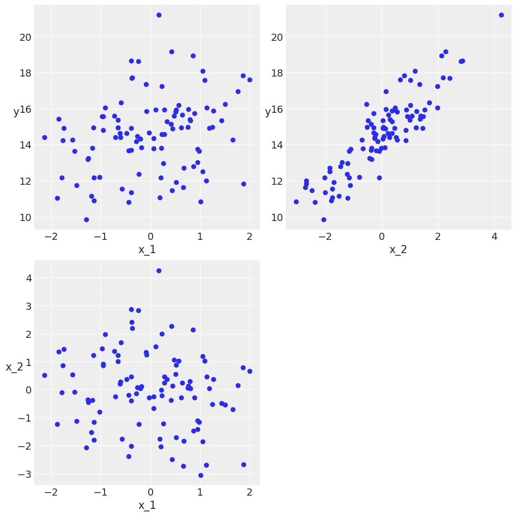
Multiple Linear regression

N = 100
alpha_real = 2.5
beta_real = jnp.array([0.9, 1.5])
eps_real = dist.Normal(loc=0, scale=0.5).sample(random.PRNGKey(0), (N,))

X = jnp.array([dist.Normal(loc=i, scale=j).sample(random.PRNGKey(i), (N,)) for i, j in zip([10, 2], [1, 1.5])]).T
X_mean = X.mean(axis=0, keepdims=True)
X_centered = X - X_mean
y = alpha_real + jnp.dot(X, beta_real) + eps_real

def scatter_plot(x, y):
    plt.figure(figsize=(10, 10))
    for idx, x_i in enumerate(x.T):
        plt.subplot(2, 2, idx+1)
        plt.scatter(x_i, y)
        plt.xlabel(f'x_{idx+1}')
        plt.ylabel(f'y', rotation=0)

    plt.subplot(2, 2, idx+2)
    plt.scatter(x[:, 0], x[:, 1])
    plt.xlabel(f'x_{idx}')
    plt.ylabel(f'x_{idx+1}', rotation=0)

scatter_plot(X_centered, y)

def model(obs=None):
    α_tmp = numpyro.sample("α_tmp", dist.Normal(loc=0, scale=10))
    β = numpyro.sample("β", dist.Normal(loc=0, scale=1), sample_shape=(2,))
    ϵ = numpyro.sample('ϵ', dist.HalfCauchy(scale=5))
                        
    μ = numpyro.deterministic('μ', α_tmp + jnp.dot(X_centered, β))
    α = numpyro.deterministic('α', α_tmp - jnp.dot(X_mean, β))
                            
    y_pred = numpyro.sample('y_pred', dist.Normal(loc=μ, scale=ϵ), obs=obs)
    

kernel = NUTS(model)
mcmc7 = MCMC(kernel, num_warmup=1000, num_samples=1000, num_chains=4, chain_method='sequential')
mcmc7.run(random.PRNGKey(seed), obs=y)

sample: 100%|████████████████████████████████████████████| 2000/2000 [00:06<00:00, 332.92it/s, 7 steps of size 7.52e-01. acc. prob=0.91]
sample: 100%|███████████████████████████████████████████| 2000/2000 [00:00<00:00, 2292.94it/s, 7 steps of size 6.92e-01. acc. prob=0.92]
sample: 100%|███████████████████████████████████████████| 2000/2000 [00:00<00:00, 3164.76it/s, 3 steps of size 7.51e-01. acc. prob=0.91]
sample: 100%|███████████████████████████████████████████| 2000/2000 [00:00<00:00, 4539.91it/s, 7 steps of size 6.91e-01. acc. prob=0.92]

varnames = ['α', 'β', 'ϵ']
az.plot_trace(mcmc7, var_names=varnames);

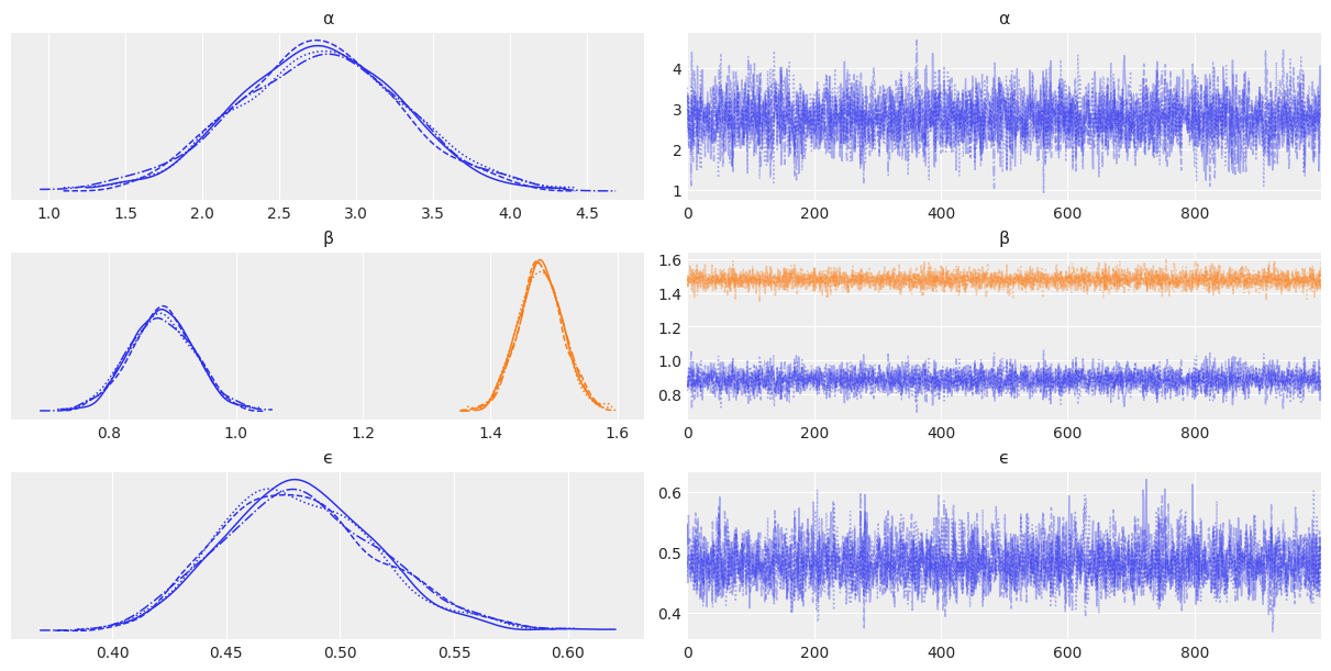
az.summary(mcmc7, var_names=varnames)

	mean	sd	hdi_3%	hdi_97%	mcse_mean	mcse_sd	ess_bulk	ess_tail	r_hat
α[0]	2.762	0.541	1.793	3.841	0.008	0.006	4249.0	2985.0	1.0
β[0]	0.882	0.052	0.781	0.976	0.001	0.001	4289.0	2991.0	1.0
β[1]	1.479	0.035	1.415	1.547	0.001	0.000	4542.0	3325.0	1.0
ϵ	0.482	0.035	0.416	0.545	0.001	0.000	4234.0	2830.0	1.0

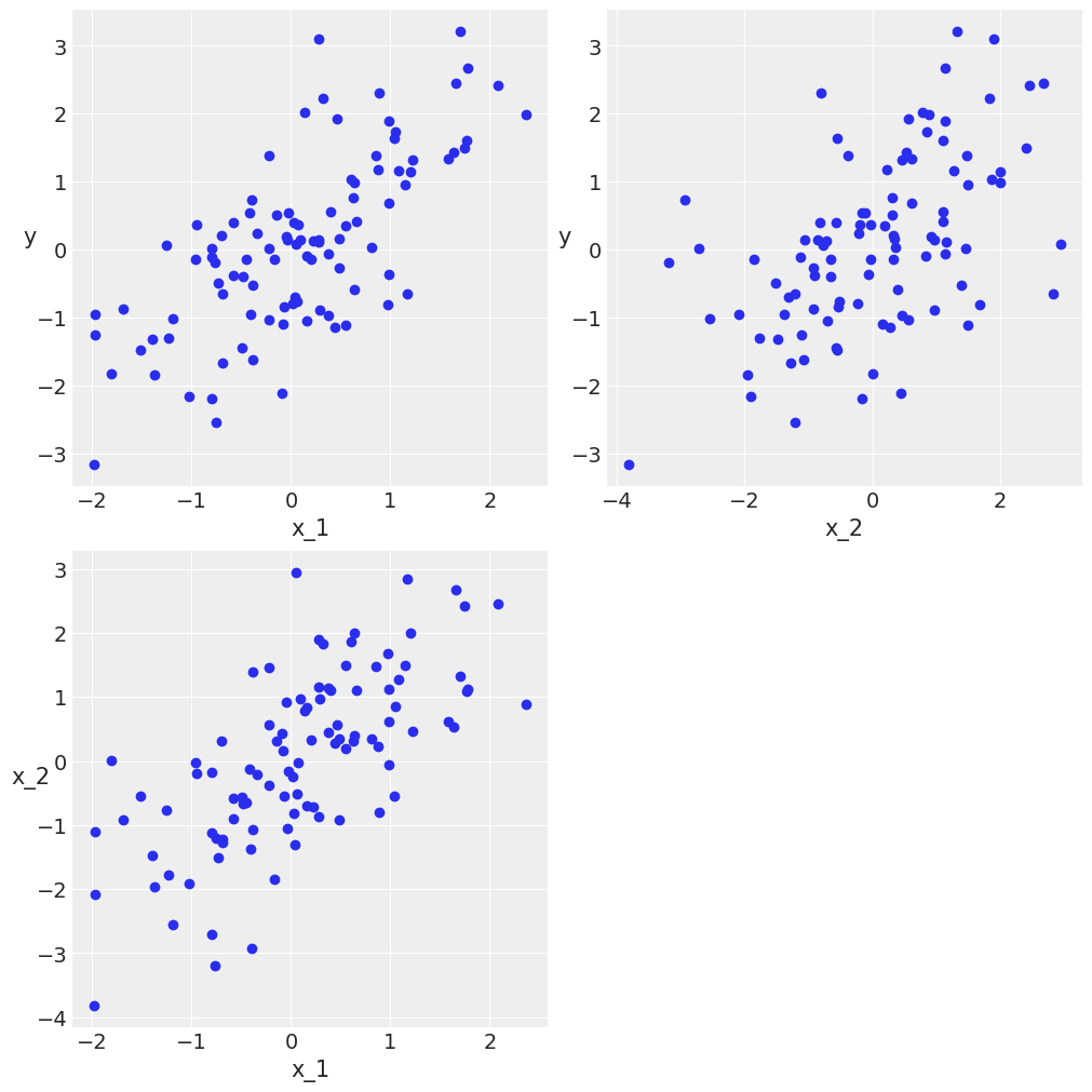
Confounding variables and redundant variables

N = 100

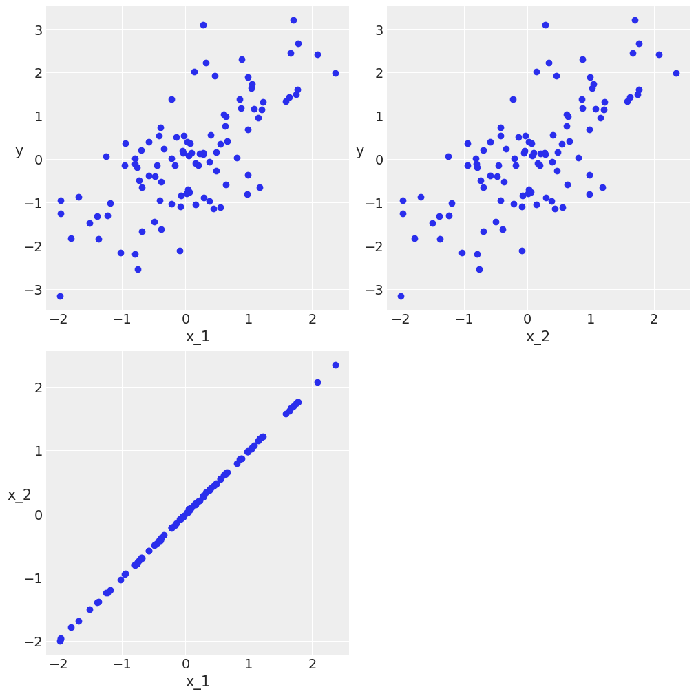
x_1 = dist.Normal().sample(random.PRNGKey(0), (N,))
x_2 = x_1 + numpyro.sample("x_2", dist.Normal(scale=1), rng_key=random.PRNGKey(1), sample_shape=(N,))
#x_2 = x_1 + np.random.normal(size=N, scale=0.01)
y = x_1 + dist.Normal().sample(random.PRNGKey(2), (N,))
X = jnp.vstack((x_1, x_2)).T

scatter_plot(X, y)

def model_x1x2(obs=None):
    α = numpyro.sample("α", dist.Normal(loc=0, scale=10))
    β1 = numpyro.sample("β1", dist.Normal(loc=0, scale=10))
    β2 = numpyro.sample("β2", dist.Normal(loc=0, scale=10))
    ϵ = numpyro.sample('ϵ', dist.HalfCauchy(scale=5))
    
    μ = α + β1 * X[:, 0] + β2 * X[:, 1]
    
    y_pred = numpyro.sample('y_pred', dist.Normal(loc=μ, scale=ϵ), obs=obs)
    
kernel = NUTS(model_x1x2)
mcmc_x1x2 = MCMC(kernel, num_warmup=1000, num_samples=1000, num_chains=4, chain_method='sequential')
mcmc_x1x2.run(random.PRNGKey(seed), obs=y)

sample: 100%|████████████████████████████████████████████| 2000/2000 [00:04<00:00, 460.12it/s, 7 steps of size 5.36e-01. acc. prob=0.92]
sample: 100%|███████████████████████████████████████████| 2000/2000 [00:00<00:00, 5674.15it/s, 7 steps of size 5.68e-01. acc. prob=0.91]
sample: 100%|███████████████████████████████████████████| 2000/2000 [00:00<00:00, 4148.05it/s, 7 steps of size 5.67e-01. acc. prob=0.91]
sample: 100%|███████████████████████████████████████████| 2000/2000 [00:00<00:00, 3189.88it/s, 7 steps of size 4.56e-01. acc. prob=0.94]

def model_x1(obs=None):
    α = numpyro.sample("α", dist.Normal(loc=0, scale=10))
    β1 = numpyro.sample("β1", dist.Normal(loc=0, scale=10))
    ϵ = numpyro.sample('ϵ', dist.HalfCauchy(scale=5))
    
    μ = α + β1 * X[:, 0]
    
    y_pred = numpyro.sample('y_pred', dist.Normal(loc=μ, scale=ϵ), obs=obs)
    
kernel = NUTS(model_x1)
mcmc_x1 = MCMC(kernel, num_warmup=1000, num_samples=1000, num_chains=4, chain_method='sequential')
mcmc_x1.run(random.PRNGKey(seed), obs=y)

sample: 100%|████████████████████████████████████████████| 2000/2000 [00:04<00:00, 499.87it/s, 1 steps of size 7.29e-01. acc. prob=0.92]
sample: 100%|███████████████████████████████████████████| 2000/2000 [00:00<00:00, 4851.33it/s, 7 steps of size 7.55e-01. acc. prob=0.92]
sample: 100%|███████████████████████████████████████████| 2000/2000 [00:00<00:00, 4453.59it/s, 7 steps of size 7.73e-01. acc. prob=0.92]
sample: 100%|███████████████████████████████████████████| 2000/2000 [00:00<00:00, 3837.34it/s, 7 steps of size 6.53e-01. acc. prob=0.95]

def model_x2(obs=None):
    α = numpyro.sample("α", dist.Normal(loc=0, scale=10))
    β2 = numpyro.sample("β2", dist.Normal(loc=0, scale=10))
    ϵ = numpyro.sample('ϵ', dist.HalfCauchy(scale=5))
    
    μ = α + β2 * X[:, 1]
    
    y_pred = numpyro.sample('y_pred', dist.Normal(loc=μ, scale=ϵ), obs=obs)
    
kernel = NUTS(model_x2)
mcmc_x2 = MCMC(kernel, num_warmup=1000, num_samples=1000, num_chains=4, chain_method='sequential')
mcmc_x2.run(random.PRNGKey(seed), obs=y)

sample: 100%|████████████████████████████████████████████| 2000/2000 [00:05<00:00, 396.51it/s, 7 steps of size 7.10e-01. acc. prob=0.93]
sample: 100%|███████████████████████████████████████████| 2000/2000 [00:00<00:00, 4994.12it/s, 7 steps of size 8.26e-01. acc. prob=0.91]
sample: 100%|███████████████████████████████████████████| 2000/2000 [00:00<00:00, 5327.92it/s, 7 steps of size 6.89e-01. acc. prob=0.93]
sample: 100%|███████████████████████████████████████████| 2000/2000 [00:00<00:00, 4916.17it/s, 7 steps of size 7.58e-01. acc. prob=0.92]

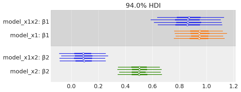
az.plot_forest([mcmc_x1x2, mcmc_x1, mcmc_x2],
               model_names=['model_x1x2', 'model_x1', 'model_x2'],
               var_names=['β1', 'β2'],
               combined=False, colors='cycle', figsize=(8, 3))

array([<AxesSubplot:title={'center':'94.0% HDI'}>], dtype=object)

# just repeating the code from a couple of cells before, but with a lower value of `scale`.
N = 100

x_1 = dist.Normal().sample(random.PRNGKey(0), (N,))
x_2 = x_1 + numpyro.sample("x_2", dist.Normal(scale=0.01), rng_key=random.PRNGKey(1), sample_shape=(N,))

y = x_1 + dist.Normal().sample(random.PRNGKey(2), (N,))
X = jnp.vstack((x_1, x_2)).T

scatter_plot(X, y)

def model_red(obs=None):
    α = numpyro.sample("α", dist.Normal(loc=0, scale=10))
    β = numpyro.sample("β", dist.Normal(loc=0, scale=10), sample_shape=(2,))
    ϵ = numpyro.sample('ϵ', dist.HalfCauchy(scale=5))
    
    μ = α + jnp.dot(X, β)
    
    y_pred = numpyro.sample('y_pred', dist.Normal(loc=μ, scale=ϵ), obs=obs)
    
kernel = NUTS(model_red)
mcmc_red = MCMC(kernel, num_warmup=1000, num_samples=1000, num_chains=4, chain_method='sequential')
mcmc_red.run(random.PRNGKey(seed), obs=y)

sample: 100%|████████████████████████████████████████████| 2000/2000 [00:03<00:00, 509.76it/s, 7 steps of size 1.31e-02. acc. prob=0.93]
sample: 100%|█████████████████████████████████████████| 2000/2000 [00:00<00:00, 2461.02it/s, 255 steps of size 1.26e-02. acc. prob=0.93]
sample: 100%|█████████████████████████████████████████| 2000/2000 [00:00<00:00, 2355.23it/s, 187 steps of size 1.12e-02. acc. prob=0.95]
sample: 100%|█████████████████████████████████████████| 2000/2000 [00:00<00:00, 2263.38it/s, 255 steps of size 1.33e-02. acc. prob=0.91]

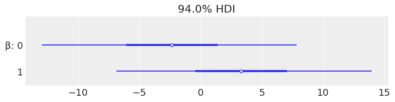
az.plot_forest(mcmc_red, var_names=['β'], combined=True, figsize=(8, 2))

array([<AxesSubplot:title={'center':'94.0% HDI'}>], dtype=object)

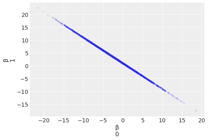
az.plot_pair(mcmc_red, var_names=['β'], scatter_kwargs={'alpha': 0.1})

<AxesSubplot:xlabel='β\n0', ylabel='β\n1'>

Masking effect variables

import numpy as np
np.random.seed(42)

N = 126
r = 0.8

x_1 = np.random.normal(size=N)
x_2 = np.random.normal(x_1, scale=(1 - r ** 2) ** 0.5)

y = np.random.normal(x_1 - x_2)
X = np.vstack((x_1, x_2)).T

x_1.shape, x_2.shape, y.shape, X.shape

((126,), (126,), (126,), (126, 2))

# N = 126
# r = 0.8

# x_1 = dist.Normal().sample(random.PRNGKey(0), (N,))
# x_2 = dist.Normal(loc=x_1, scale=(1 - r ** 2) ** 0.5).sample(random.PRNGKey(0), (N,))

# y = dist.Normal(loc=(x_1 - x_2)).sample(random.PRNGKey(2), (N,))
# X = jnp.vstack((x_1, x_2)).T

# x_1.shape, x_2.shape, y.shape, X.shape

# TODO: Fix errors regarding shape of x_1.shape, x_2.shape, y.shape, X.shape above
# scatter_plot(X, y)

def model_x1x2(obs=None):
    α = numpyro.sample("α", dist.Normal(loc=0, scale=10))
    β1 = numpyro.sample("β1", dist.Normal(loc=0, scale=10))
    β2 = numpyro.sample("β2", dist.Normal(loc=0, scale=10))
    ϵ = numpyro.sample('ϵ', dist.HalfCauchy(scale=5))
    
    μ = α + β1 * X[:, 0] + β2 * X[:, 1]
    
    y_pred = numpyro.sample('y_pred', dist.Normal(loc=μ, scale=ϵ), obs=obs)
    
kernel = NUTS(model_x1x2)
mcmc_x1x2 = MCMC(kernel, num_warmup=1000, num_samples=1000, num_chains=4, chain_method='sequential')
mcmc_x1x2.run(random.PRNGKey(seed), obs=y)

sample: 100%|███████████████████████████████████████████| 2000/2000 [00:05<00:00, 363.66it/s, 15 steps of size 3.35e-01. acc. prob=0.94]
sample: 100%|██████████████████████████████████████████| 2000/2000 [00:00<00:00, 4584.59it/s, 15 steps of size 4.12e-01. acc. prob=0.91]
sample: 100%|██████████████████████████████████████████| 2000/2000 [00:00<00:00, 4568.60it/s, 15 steps of size 3.07e-01. acc. prob=0.94]
sample: 100%|██████████████████████████████████████████| 2000/2000 [00:00<00:00, 4706.65it/s, 15 steps of size 3.45e-01. acc. prob=0.93]

def model_x1(obs=None):
    α = numpyro.sample("α", dist.Normal(loc=0, scale=10))
    β1 = numpyro.sample("β1", dist.Normal(loc=0, scale=10))
    ϵ = numpyro.sample('ϵ', dist.HalfCauchy(scale=5))
    
    μ = α + β1 * X[:, 0]
    
    y_pred = numpyro.sample('y_pred', dist.Normal(loc=μ, scale=ϵ), obs=obs)
    
kernel = NUTS(model_x1)
mcmc_x1 = MCMC(kernel, num_warmup=1000, num_samples=1000, num_chains=4, chain_method='sequential')
mcmc_x1.run(random.PRNGKey(seed), obs=y)

sample: 100%|████████████████████████████████████████████| 2000/2000 [00:04<00:00, 475.11it/s, 3 steps of size 7.82e-01. acc. prob=0.91]
sample: 100%|███████████████████████████████████████████| 2000/2000 [00:00<00:00, 3732.54it/s, 7 steps of size 6.70e-01. acc. prob=0.95]
sample: 100%|███████████████████████████████████████████| 2000/2000 [00:00<00:00, 4749.03it/s, 7 steps of size 7.28e-01. acc. prob=0.92]
sample: 100%|███████████████████████████████████████████| 2000/2000 [00:00<00:00, 5351.96it/s, 7 steps of size 8.04e-01. acc. prob=0.91]

def model_x2(obs=None):
    α = numpyro.sample("α", dist.Normal(loc=0, scale=10))
    β2 = numpyro.sample("β2", dist.Normal(loc=0, scale=10))
    ϵ = numpyro.sample('ϵ', dist.HalfCauchy(scale=5))
    
    μ = α + β2 * X[:, 1]
    
    y_pred = numpyro.sample('y_pred', dist.Normal(loc=μ, scale=ϵ), obs=obs)
    
kernel = NUTS(model_x2)
mcmc_x2 = MCMC(kernel, num_warmup=1000, num_samples=1000, num_chains=4, chain_method='sequential')
mcmc_x2.run(random.PRNGKey(seed), obs=y)

sample: 100%|████████████████████████████████████████████| 2000/2000 [00:04<00:00, 406.93it/s, 7 steps of size 7.51e-01. acc. prob=0.92]
sample: 100%|███████████████████████████████████████████| 2000/2000 [00:00<00:00, 4098.25it/s, 3 steps of size 8.57e-01. acc. prob=0.90]
sample: 100%|███████████████████████████████████████████| 2000/2000 [00:00<00:00, 4698.66it/s, 3 steps of size 7.31e-01. acc. prob=0.92]
sample: 100%|███████████████████████████████████████████| 2000/2000 [00:00<00:00, 4068.20it/s, 7 steps of size 7.16e-01. acc. prob=0.93]

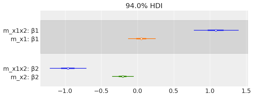
az.plot_forest([mcmc_x1x2, mcmc_x1, mcmc_x2],
               model_names=['m_x1x2', 'm_x1', 'm_x2'],
               var_names=['β1', 'β2'],
               combined=True, colors='cycle', figsize=(8, 3))

array([<AxesSubplot:title={'center':'94.0% HDI'}>], dtype=object)

Variable variance

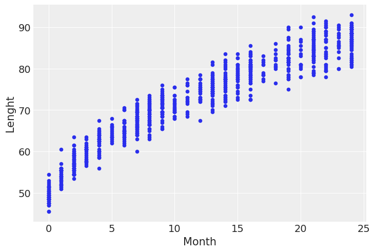
data = pd.read_csv('../data/babies.csv')
data.plot.scatter('Month', 'Lenght')

<AxesSubplot:xlabel='Month', ylabel='Lenght'>

def model_vv(obs=None):
    α = numpyro.sample("α", dist.Normal(scale=10))
    β = numpyro.sample("β", dist.Normal(scale=10))
    γ = numpyro.sample('γ', dist.HalfNormal(scale=10))
    δ = numpyro.sample('δ', dist.HalfNormal(scale=10))
    
    x_shared = (data.Month.values * 1.)  # TODO: Understand better what theano.shared() is doing
    
    μ = numpyro.deterministic('μ', α + β * x_shared**0.5)
    ϵ = numpyro.deterministic('ϵ', γ + δ * x_shared)
    
    y_pred = numpyro.sample('y_pred', dist.Normal(loc=μ, scale=ϵ), obs=obs)
    
kernel = NUTS(model_vv)
mcmc_vv = MCMC(kernel, num_warmup=1000, num_samples=1000, num_chains=4, chain_method='sequential')
mcmc_vv.run(random.PRNGKey(seed), obs=jnp.asarray(data.Lenght))

sample: 100%|███████████████████████████████████████████| 2000/2000 [00:04<00:00, 459.54it/s, 15 steps of size 2.88e-01. acc. prob=0.92]
sample: 100%|██████████████████████████████████████████| 2000/2000 [00:00<00:00, 3869.99it/s, 15 steps of size 2.56e-01. acc. prob=0.95]
sample: 100%|███████████████████████████████████████████| 2000/2000 [00:00<00:00, 4245.70it/s, 7 steps of size 2.51e-01. acc. prob=0.94]
sample: 100%|██████████████████████████████████████████| 2000/2000 [00:00<00:00, 4319.11it/s, 15 steps of size 3.14e-01. acc. prob=0.92]

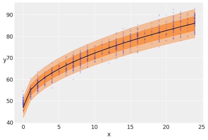
plt.plot(data.Month, data.Lenght, 'C0.', alpha=0.1)

μ_m = mcmc_vv.get_samples()['μ'].mean(0)
ϵ_m = mcmc_vv.get_samples()['ϵ'].mean(0)

plt.plot(data.Month, μ_m, c='k')
plt.fill_between(data.Month, μ_m + 1 * ϵ_m, μ_m -
                 1 * ϵ_m, alpha=0.6, color='C1')
plt.fill_between(data.Month, μ_m + 2 * ϵ_m, μ_m -
                 2 * ϵ_m, alpha=0.4, color='C1')

plt.xlabel('x')
plt.ylabel('y', rotation=0)

Text(0, 0.5, 'y')

# x_shared.set_value([0.5]) -- Does not seem to be required
pred = Predictive(model=mcmc_vv.sampler.model, posterior_samples=mcmc_vv.get_samples(), return_sites=['y_pred'])
ppc = pred(random.PRNGKey(seed))
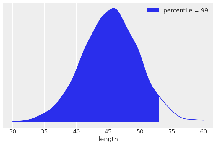
y_ppc = ppc['y_pred'][:, 0]

# https://github.com/aloctavodia/BAP/issues/69
ref = 53
# density, l, u = az._fast_kde(y_ppc) # TODO: _fast_kde deprecated. Need to investigate further 
grid, density = az.kde(y_ppc)
l, u = min(grid), max(grid)
print(l, u)
x_ = jnp.linspace(30, 60, density.shape[0])
print(density.shape)

38.56563255563378 54.932746198028326
(512,)

plt.plot(x_, density)

percentile = int(sum(y_ppc <= ref) / len(y_ppc) * 100)

plt.fill_between(x_[x_ < ref], density[x_ < ref],
                 label='percentile = {:2d}'.format(percentile))

plt.xlabel('length')
plt.yticks([])
plt.legend()

<matplotlib.legend.Legend at 0x7fb4649e6490>

x_4 = ans[ans.group == 'IV']['x'].values
y_4 = ans[ans.group == 'IV']['y'].values

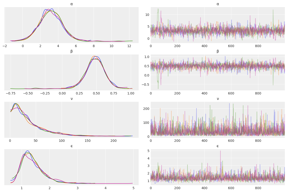
def model_t2(obs=None):
    α = numpyro.sample("α", dist.Normal(loc=0, scale=100))
    β = numpyro.sample("β", dist.Normal(loc=0, scale=1))
    ϵ = numpyro.sample('ϵ', dist.HalfCauchy(scale=5))
    ν = numpyro.sample('ν', dist.Exponential(rate=1/30))
#     ν = numpyro.sample('ν', dist.Gamma(concentration=20, rate=15))
#     ν = numpyro.sample('ν', dist.Gamma(concentration=2, rate=0.1))
    
    y_pred = numpyro.sample('y_pred', dist.StudentT(df=ν, loc=α + β * x_4, scale=ϵ), obs=obs)
    
kernel = NUTS(model_t2)
mcmc_t2 = MCMC(kernel, num_warmup=1000, num_samples=1000, num_chains=4, chain_method='sequential')
mcmc_t2.run(random.PRNGKey(seed), obs=y_4)

sample: 100%|███████████████████████████████████████████| 2000/2000 [00:03<00:00, 609.61it/s, 15 steps of size 2.42e-01. acc. prob=0.86]
sample: 100%|███████████████████████████████████████████| 2000/2000 [00:00<00:00, 5241.23it/s, 7 steps of size 2.59e-01. acc. prob=0.89]
sample: 100%|██████████████████████████████████████████| 2000/2000 [00:00<00:00, 5162.71it/s, 15 steps of size 2.16e-01. acc. prob=0.91]
sample: 100%|██████████████████████████████████████████| 2000/2000 [00:00<00:00, 4200.82it/s, 15 steps of size 1.59e-01. acc. prob=0.94]

az.plot_trace(mcmc_t2, compact=False)

array([[<AxesSubplot:title={'center':'α'}>,
        <AxesSubplot:title={'center':'α'}>],
       [<AxesSubplot:title={'center':'β'}>,
        <AxesSubplot:title={'center':'β'}>],
       [<AxesSubplot:title={'center':'ν'}>,
        <AxesSubplot:title={'center':'ν'}>],
       [<AxesSubplot:title={'center':'ϵ'}>,
        <AxesSubplot:title={'center':'ϵ'}>]], dtype=object)

az.summary(mcmc_t2)

	mean	sd	hdi_3%	hdi_97%	mcse_mean	mcse_sd	ess_bulk	ess_tail	r_hat
α	3.190	1.399	0.681	5.748	0.042	0.035	1362.0	1362.0	1.0
β	0.479	0.148	0.221	0.755	0.004	0.003	1403.0	1376.0	1.0
ν	35.472	31.417	0.905	93.961	0.595	0.431	2491.0	2332.0	1.0
ϵ	1.387	0.401	0.779	2.168	0.010	0.007	1926.0	1621.0	1.0

previous

Chapter 2. Programming Probabilistically

next

Chapter 4. Generalizing Linear Models