Chapter 2. Programming Probabilistically
import os
import warnings

import arviz as az
import matplotlib.pyplot as plt
import pandas as pd
from scipy.interpolate import BSpline
from scipy.stats import gaussian_kde

import jax.numpy as jnp
from jax import random, vmap

import numpyro
import numpyro.distributions as dist
import numpyro.optim as optim

from numpyro.infer import MCMC, NUTS, HMC, Predictive
from numpyro.diagnostics import hpdi, print_summary
from numpyro.infer import Predictive, SVI, Trace_ELBO, init_to_value
from numpyro.infer.autoguide import AutoLaplaceApproximation

seed=4321

if "SVG" in os.environ:
    %config InlineBackend.figure_formats = ["svg"]
warnings.formatwarning = lambda message, category, *args, **kwargs: "{}: {}\n".format(
    category.__name__, message
)
az.style.use("arviz-darkgrid")
numpyro.set_platform("cpu") # or "gpu", "tpu" depending on system
numpyro primer
trials = 4
theta_real = 0.35  # unknown value in a real experiment
# data = stats.bernoulli.rvs(p=theta_real, size=trials)
data = dist.Bernoulli(probs=theta_real).sample(random.PRNGKey(1), (trials,))
data
DeviceArray([0, 1, 0, 0], dtype=int32)
def model(data):
    # a priori
    θ = numpyro.sample('θ', dist.Beta(1., 1.))
    # likelihood
    numpyro.sample('y', dist.Bernoulli(probs=θ), obs=data)

kernel = NUTS(model)
mcmc = MCMC(kernel, num_warmup=500, num_samples=1500, num_chains=2)
mcmc.run(random.PRNGKey(1), data=data)
UserWarning: There are not enough devices to run parallel chains: expected 2 but got 1. Chains will be drawn sequentially. If you are running MCMC in CPU, consider using `numpyro.set_host_device_count(2)` at the beginning of your program. You can double-check how many devices are available in your system using `jax.local_device_count()`.
sample: 100%|███████████████████████████| 2000/2000 [00:02<00:00, 797.62it/s, 1 steps of size 9.83e-01. acc. prob=0.92]
sample: 100%|██████████████████████████| 2000/2000 [00:00<00:00, 7209.50it/s, 3 steps of size 1.13e+00. acc. prob=0.90]
Summarizing the posterior
az.plot_trace(az.from_numpyro(mcmc), compact=False)
plt.show()
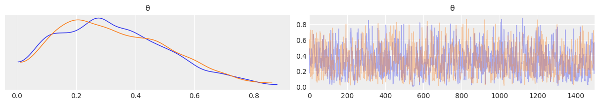
mcmc.print_summary()
mean std median 5.0% 95.0% n_eff r_hat
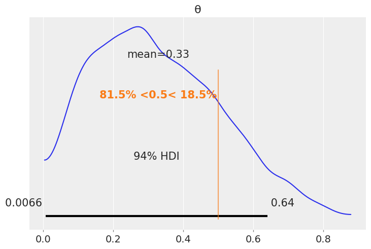
θ 0.33 0.18 0.31 0.05 0.61 1051.12 1.00
Number of divergences: 0
Posterior-based decisions
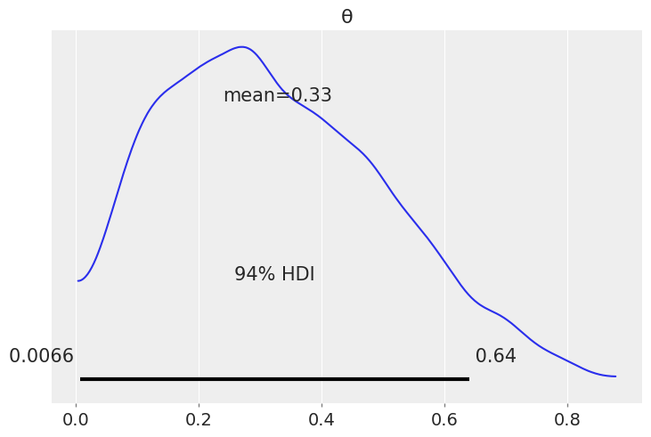
az.plot_posterior(az.from_numpyro(mcmc))
plt.show()
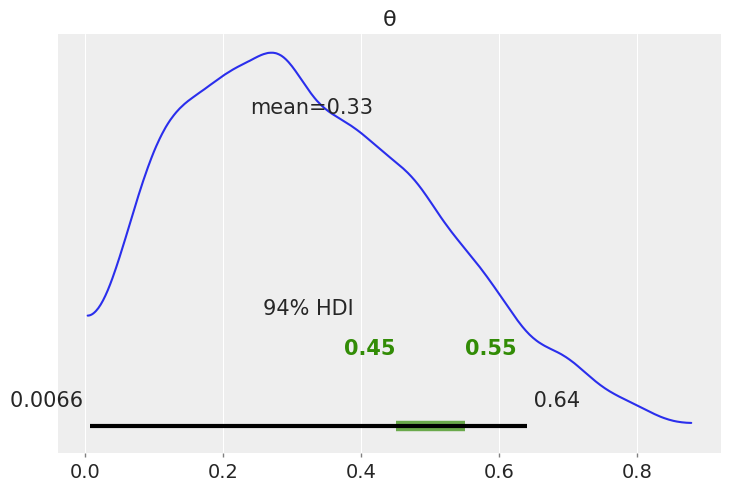
az.plot_posterior(az.from_numpyro(mcmc), rope=[0.45, .55])
<AxesSubplot:title={'center':'θ'}>
az.plot_posterior(az.from_numpyro(mcmc), ref_val=0.5)
<AxesSubplot:title={'center':'θ'}>
mcmc.get_samples(group_by_chain=True)
{'θ': DeviceArray([[0.17285858, 0.32812756, 0.48738322, ..., 0.16604272,
               0.4787685 , 0.5638707 ],
              [0.57522225, 0.6004805 , 0.4808577 , ..., 0.22368269,
               0.21266927, 0.21266927]], dtype=float32)}
grid = jnp.linspace(start=0, stop=1, num=200)
θ_pos = mcmc.get_samples()["θ"]
lossf_a = [jnp.mean(abs(i - θ_pos)) for i in grid]
lossf_b = [jnp.mean((i - θ_pos)**2) for i in grid]

for lossf, c in zip([lossf_a, lossf_b], ['C0', 'C1']):
    mini = jnp.argmin(jnp.asarray(lossf))
    plt.plot(grid, lossf, c)
    plt.plot(grid[mini], lossf[mini], 'o', color=c)
    plt.annotate('{:.2f}'.format(grid[mini]),
                 (grid[mini], lossf[mini] + 0.03), color=c)
    plt.yticks([])
    plt.xlabel(r'$\hat \theta$')
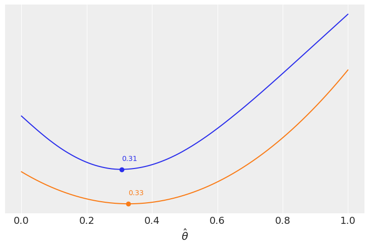
jnp.mean(θ_pos), jnp.median(θ_pos)
(DeviceArray(0.32869053, dtype=float32),
 DeviceArray(0.30531082, dtype=float32))
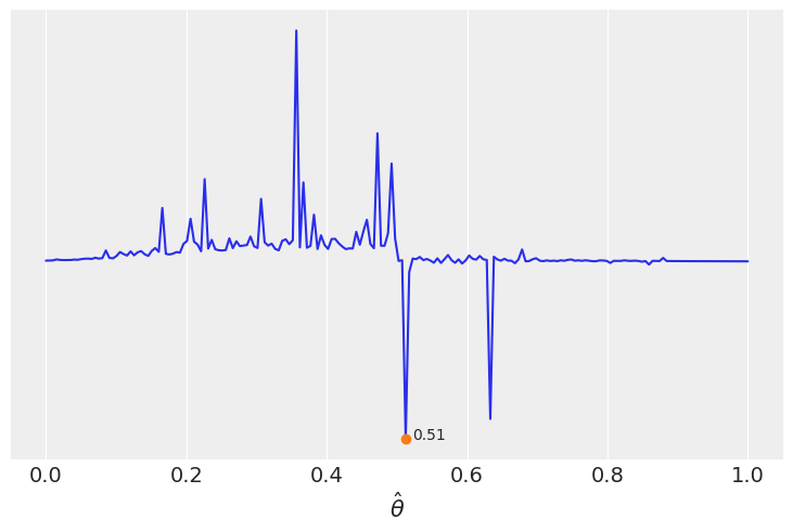
lossf = []
for i in grid:
    if i < 0.5:
        f = jnp.mean(jnp.pi * θ_pos / jnp.abs(i - θ_pos))
    else:
        f = jnp.mean(1 / (i - θ_pos))
    lossf.append(f)

mini = jnp.argmin(jnp.asarray(lossf))
plt.plot(grid, lossf)
plt.plot(grid[mini], lossf[mini], 'o')
plt.annotate('{:.2f}'.format(grid[mini]),
             (grid[mini] + 0.01, lossf[mini] + 0.1))
plt.yticks([])
plt.xlabel(r'$\hat \theta$')
Text(0.5, 0, '$\\hat \\theta$')
Gaussian inferences
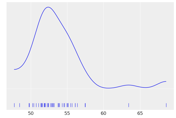
data = pd.read_csv('../data/chemical_shifts.csv', header=None)
data.head()
| 0 | |
|---|---|
| 0 | 51.06 |
| 1 | 55.12 |
| 2 | 53.73 |
| 3 | 50.24 |
| 4 | 52.05 |
data = jnp.asarray(data)
data.shape
(48, 1)
az.plot_kde(data, rug=True)
plt.yticks([0], alpha=0)
([<matplotlib.axis.YTick at 0x1272bdf40>], [Text(0, 0, '')])
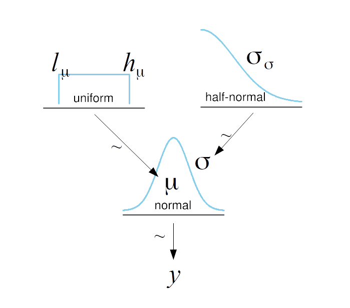
def model(N=100, obs=None):
    μ = numpyro.sample('μ', dist.Uniform(low=40., high=70.))
    σ = numpyro.sample('σ', dist.HalfNormal(scale=10.))
    with numpyro.plate("N", N):
        numpyro.sample('y', dist.Normal(loc=μ, scale=σ), obs=obs)


kernel = NUTS(model)
mcmc2 = MCMC(kernel, num_warmup=500, num_samples=500, num_chains=2)
mcmc2.run(random.PRNGKey(seed), obs=data)
UserWarning: There are not enough devices to run parallel chains: expected 2 but got 1. Chains will be drawn sequentially. If you are running MCMC in CPU, consider using `numpyro.set_host_device_count(2)` at the beginning of your program. You can double-check how many devices are available in your system using `jax.local_device_count()`.
sample: 100%|███████████████████████████| 1000/1000 [00:02<00:00, 406.78it/s, 1 steps of size 7.91e-01. acc. prob=0.89]
sample: 100%|██████████████████████████| 1000/1000 [00:00<00:00, 6035.36it/s, 3 steps of size 6.60e-01. acc. prob=0.93]
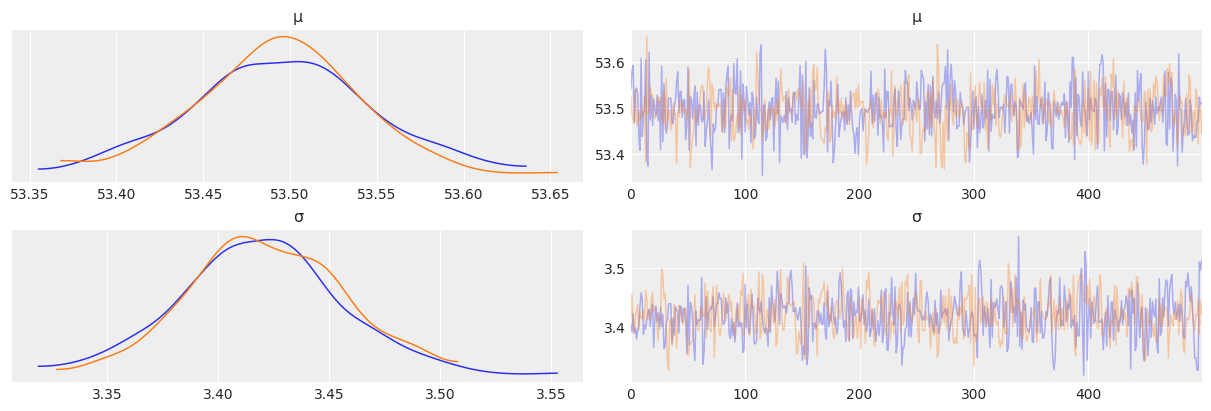
az.plot_trace(az.from_numpyro(mcmc2), compact=False)
plt.show()
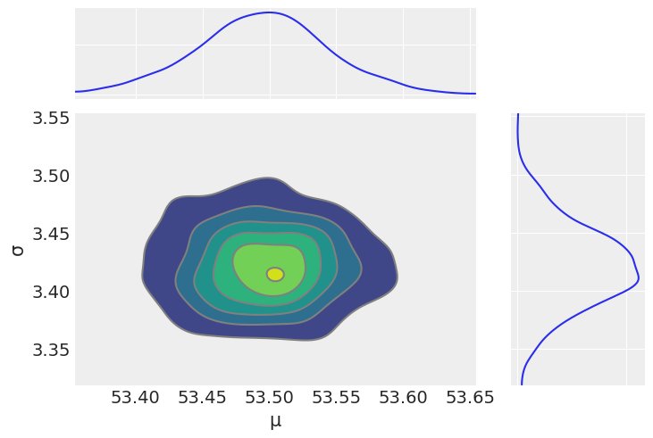
az.plot_joint(az.from_numpyro(mcmc2), var_names=['μ', 'σ'], kind='kde', fill_last=False)
UserWarning: plot_joint will be deprecated. Please use plot_pair instead.
array([<AxesSubplot:xlabel='μ', ylabel='σ'>, <AxesSubplot:>,
       <AxesSubplot:>], dtype=object)
mcmc2.print_summary()
                mean       std    median      5.0%     95.0%     n_eff     r_hat
         μ     53.49      0.05     53.50     53.40     53.57    787.94      1.00
         σ      3.42      0.04      3.42      3.36      3.48    685.76      1.00

Number of divergences: 0
az.summary(mcmc2)
| mean | sd | hdi_3% | hdi_97% | mcse_mean | mcse_sd | ess_bulk | ess_tail | r_hat | |
|---|---|---|---|---|---|---|---|---|---|
| μ | 53.495 | 0.049 | 53.405 | 53.594 | 0.002 | 0.001 | 795.0 | 675.0 | 1.01 |
| σ | 3.420 | 0.035 | 3.356 | 3.491 | 0.001 | 0.001 | 693.0 | 579.0 | 1.00 |
prior = Predictive(mcmc2.sampler.model, num_samples=10)
prior_p = prior(random.PRNGKey(seed), obs=data)
pred = Predictive(model=mcmc2.sampler.model, posterior_samples=mcmc2.get_samples(), return_sites=['y'])
post_p = pred(random.PRNGKey(seed), N=100)
# post_p['y'] = post_p['y'].squeeze()
# post_p['y'] = jnp.expand_dims(post_p['y'], axis=1) --> Seems line not needed
post_p['y'].shape
(1000, 100)
post_p['y'] = post_p['y'][:50]
post_p['y'].shape
(50, 100)
jnp.sort(post_p['y'][0])
DeviceArray([44.29414 , 44.349854, 46.441837, 46.689426, 46.796425,
             47.03588 , 47.583427, 47.596024, 48.212406, 48.726635,
             48.813835, 48.84052 , 49.055523, 49.085613, 49.60701 ,
             49.714584, 49.80934 , 49.83368 , 49.943848, 50.031883,
             50.160152, 50.25194 , 50.320923, 50.334843, 50.518284,
             50.518463, 50.6463  , 50.69864 , 50.728085, 50.96986 ,
             51.064117, 51.330784, 51.572712, 51.629684, 51.821022,
             51.835228, 51.87946 , 51.93214 , 52.314796, 52.3805  ,
             52.59526 , 52.771126, 52.853275, 52.88644 , 53.019768,
             53.135284, 53.27581 , 53.30327 , 53.48876 , 53.51001 ,
             53.626865, 53.722065, 53.72291 , 53.811417, 53.82796 ,
             53.831795, 53.83189 , 53.83466 , 54.084534, 54.088604,
             54.338524, 54.603535, 54.712193, 54.74976 , 54.75797 ,
             54.77956 , 54.86422 , 54.87436 , 54.945034, 54.96186 ,
             55.11813 , 55.122982, 55.267242, 55.4409  , 55.642887,
             55.657356, 55.68466 , 55.780605, 55.79514 , 56.42554 ,
             56.570297, 56.609188, 56.980118, 57.09482 , 57.193207,
             57.202858, 57.915466, 57.950962, 57.98787 , 57.992737,
             58.044582, 58.31988 , 58.68991 , 59.050575, 59.08069 ,
             59.140976, 59.159565, 60.87754 , 61.32518 , 62.033207],            dtype=float32)
# samples = az.from_numpyro(mcmc2, prior=prior_p, posterior_predictive=post_p)
samples = az.from_numpyro(mcmc2, prior=prior_p, posterior_predictive=post_p) # Priop p seems not required.
# az.summary(samples)
WARNING:arviz.data.io_numpyro:posterior predictive shape not compatible with number of chains and draws. This can mean that some draws or even whole chains are not represented.
samples.groups()
['posterior',
 'posterior_predictive',
 'log_likelihood',
 'sample_stats',
 'prior',
 'prior_predictive',
 'observed_data']
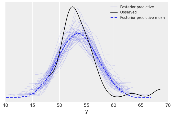
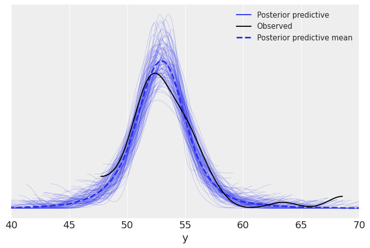
fig, ax = plt.subplots()
for i in post_p['y']:
    ax = az.plot_kde(i, ax=ax, plot_kwargs={'alpha': 0.05})
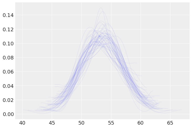
az.plot_ppc(samples, mean=True, observed=True)
plt.xlim(40, 70)
(40.0, 70.0)
Robust inferences
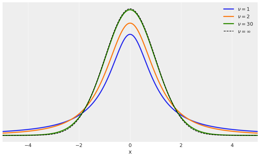
plt.figure(figsize=(10, 6))
x_values = jnp.linspace(start=-10, stop=10, num=500)
for df in [1, 2, 30]:
    distri = dist.StudentT(df)
    x_pdf = jnp.exp(distri.log_prob(x_values))
    plt.plot(x_values, x_pdf, label=fr'$\nu = {df}$', lw=3)

x_pdf = jnp.exp(dist.Normal().log_prob(x_values))
plt.plot(x_values, x_pdf, 'k--', label=r'$\nu = \infty$')
plt.xlabel('x')
plt.yticks([])
plt.legend()
plt.xlim(-5, 5)
(-5.0, 5.0)
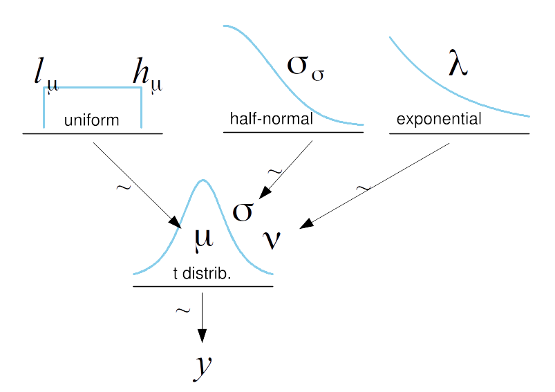
def model(N=100, obs=None):
    μ = numpyro.sample('μ', dist.Uniform(low=40., high=75.))
    σ = numpyro.sample('σ', dist.HalfNormal(scale=10.))
    ν = numpyro.sample('ν', dist.Exponential(rate=1/30))

    with numpyro.plate("N", N):
        numpyro.sample('y', dist.StudentT(ν, loc=μ, scale=σ), obs=obs)


kernel = NUTS(model)
mcmc3 = MCMC(kernel, num_warmup=500, num_samples=500, num_chains=2)
mcmc3.run(random.PRNGKey(seed), obs=data)
UserWarning: There are not enough devices to run parallel chains: expected 2 but got 1. Chains will be drawn sequentially. If you are running MCMC in CPU, consider using `numpyro.set_host_device_count(2)` at the beginning of your program. You can double-check how many devices are available in your system using `jax.local_device_count()`.
sample: 100%|███████████████████████████| 1000/1000 [00:02<00:00, 353.77it/s, 7 steps of size 5.48e-01. acc. prob=0.93]
sample: 100%|██████████████████████████| 1000/1000 [00:00<00:00, 3965.46it/s, 3 steps of size 6.52e-01. acc. prob=0.90]
az.plot_trace(az.from_numpyro(mcmc3), compact=False)
plt.show()
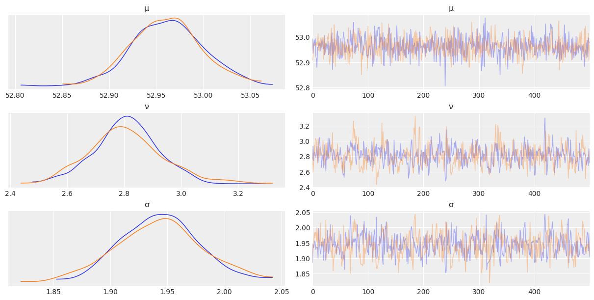
az.summary(mcmc3)
| mean | sd | hdi_3% | hdi_97% | mcse_mean | mcse_sd | ess_bulk | ess_tail | r_hat | |
|---|---|---|---|---|---|---|---|---|---|
| μ | 52.962 | 0.037 | 52.897 | 53.039 | 0.001 | 0.001 | 1085.0 | 748.0 | 1.00 |
| ν | 2.809 | 0.125 | 2.577 | 3.037 | 0.006 | 0.005 | 380.0 | 429.0 | 1.00 |
| σ | 1.944 | 0.036 | 1.880 | 2.017 | 0.002 | 0.001 | 421.0 | 444.0 | 1.01 |
prior = Predictive(mcmc3.sampler.model, num_samples=10)
prior_p = prior(random.PRNGKey(seed), obs=data)

pred = Predictive(model=mcmc3.sampler.model, posterior_samples=mcmc3.get_samples(), return_sites=['y'])
post_p = pred(random.PRNGKey(seed), N=100)
post_p['y'] = post_p['y'][:100]
samples = az.from_numpyro(mcmc3, prior=prior_p, posterior_predictive=post_p) ## CHECK THIS
WARNING:arviz.data.io_numpyro:posterior predictive shape not compatible with number of chains and draws. This can mean that some draws or even whole chains are not represented.
az.plot_ppc(samples, mean=True, observed=True, color='C0')
plt.xlim(40, 70)
(40.0, 70.0)
Tips example
tips = pd.read_csv('../data/tips.csv')
tips.tail()
| total_bill | tip | sex | smoker | day | time | size | |
|---|---|---|---|---|---|---|---|
| 239 | 29.03 | 5.92 | Male | No | Sat | Dinner | 3 |
| 240 | 27.18 | 2.00 | Female | Yes | Sat | Dinner | 2 |
| 241 | 22.67 | 2.00 | Male | Yes | Sat | Dinner | 2 |
| 242 | 17.82 | 1.75 | Male | No | Sat | Dinner | 2 |
| 243 | 18.78 | 3.00 | Female | No | Thur | Dinner | 2 |
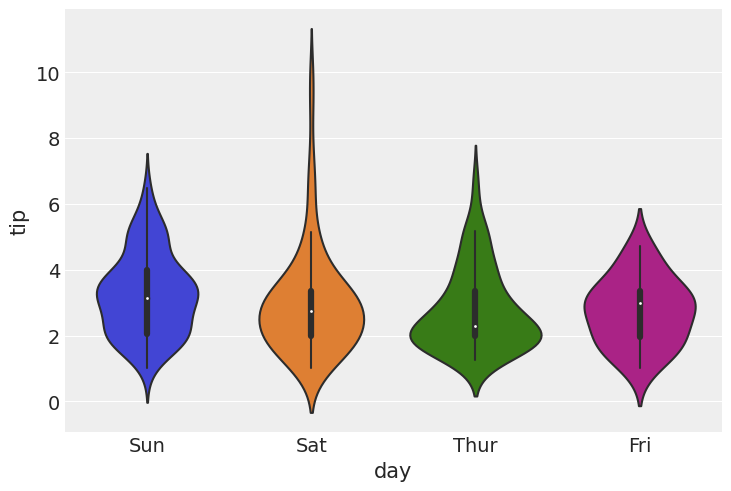
##### TODO: Violin plot with arviz
import seaborn as sns
sns.violinplot(x='day', y='tip', data=tips)
<AxesSubplot:xlabel='day', ylabel='tip'>
tip = tips['tip'].values
idx = pd.Categorical(tips['day'],
                     categories=['Thur', 'Fri', 'Sat', 'Sun']).codes
groups = len(jnp.unique(idx))
def model(N=len(idx), obs=None):
    μ = numpyro.sample('μ', dist.Normal(loc=0., scale=10.), sample_shape=(groups,))
    σ = numpyro.sample('σ', dist.HalfNormal(scale=10.), sample_shape=(groups,))

    with numpyro.plate("N", N):
        numpyro.sample('y', dist.Normal(loc=μ[idx], scale=σ[idx]), obs=obs)


kernel = NUTS(model)
mcmc4 = MCMC(kernel, num_warmup=1000, num_samples=4000, num_chains=2)
mcmc4.run(random.PRNGKey(seed), obs=tip)
UserWarning: There are not enough devices to run parallel chains: expected 2 but got 1. Chains will be drawn sequentially. If you are running MCMC in CPU, consider using `numpyro.set_host_device_count(2)` at the beginning of your program. You can double-check how many devices are available in your system using `jax.local_device_count()`.
sample: 100%|██████████████████████████| 5000/5000 [00:03<00:00, 1634.51it/s, 7 steps of size 6.41e-01. acc. prob=0.90]
sample: 100%|██████████████████████████| 5000/5000 [00:00<00:00, 5434.91it/s, 7 steps of size 5.79e-01. acc. prob=0.91]
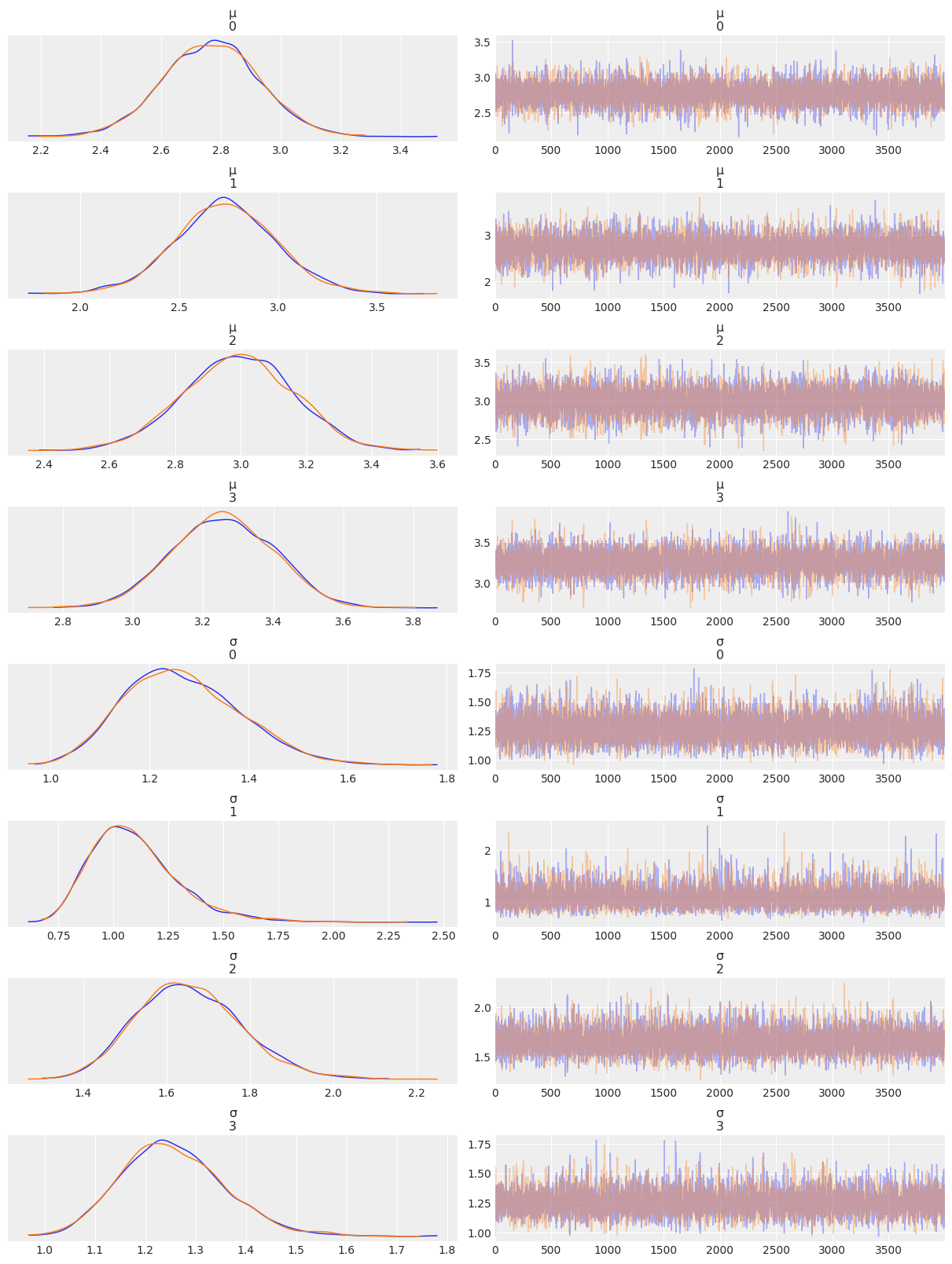
az.plot_trace(az.from_numpyro(mcmc4), compact=False)
plt.show()
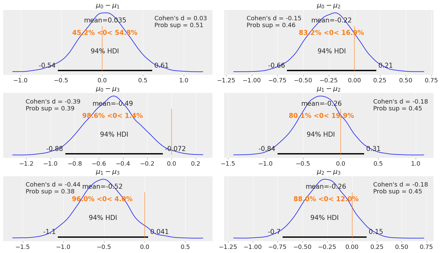
distri = dist.Normal()

_, ax = plt.subplots(3, 2, figsize=(14, 8), constrained_layout=True)

comparisons = [(i, j) for i in range(4) for j in range(i+1, 4)]
pos = [(k, l) for k in range(3) for l in (0, 1)]

for (i, j), (k, l) in zip(comparisons, pos):
    means_diff = mcmc4.get_samples()['μ'][:, i] - mcmc4.get_samples()['μ'][:, j]
    d_cohen = (means_diff / jnp.sqrt((mcmc4.get_samples()['σ'][:, i]**2 + mcmc4.get_samples()['σ'][:, j]**2) / 2)).mean()
    ps = distri.cdf(d_cohen/(2**0.5))
#     import pdb;pdb.set_trace()
    means_diff = jnp.asarray(means_diff)
    az.plot_posterior(means_diff.copy(), ref_val=0, ax=ax[k, l])
    ax[k, l].set_title(f'$\mu_{i}-\mu_{j}$')
    ax[k, l].plot(
        0, label=f"Cohen's d = {d_cohen:.2f}\nProb sup = {ps:.2f}", alpha=0)
    ax[k, l].legend()
Hierarchical Models
N_samples = [30, 30, 30]
G_samples = [18, 18, 18]  # [3, 3, 3]  [18, 3, 3]
N_samples[0]
30
group_idx = jnp.repeat(jnp.arange(len(N_samples)), N_samples[0])
data = []
for i in range(0, len(N_samples)):
    data.extend(jnp.repeat(jnp.asarray([1, 0]), jnp.asarray([G_samples[i], N_samples[i]-G_samples[i]])))
data = jnp.asarray(data)
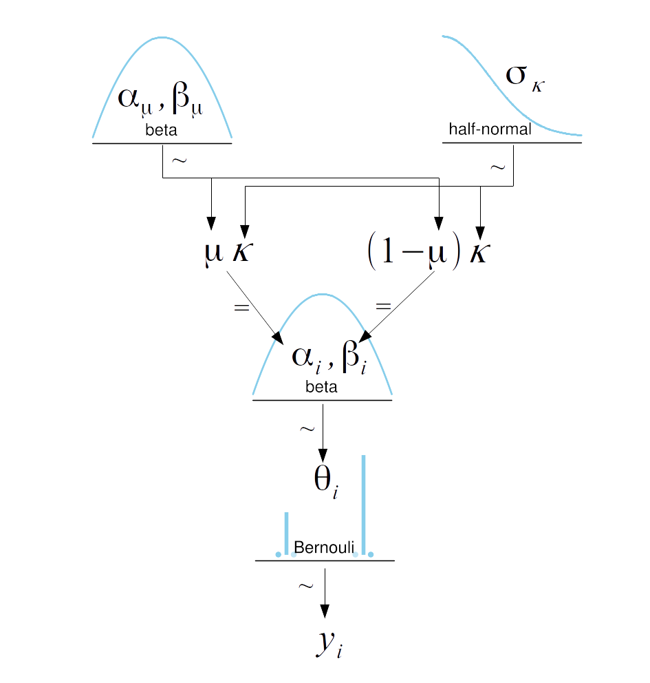
def model(obs=None):
    μ = numpyro.sample('μ', dist.Beta(1.,1.))
    κ = numpyro.sample('κ', dist.HalfNormal(scale=10.))
    θ = numpyro.sample('θ', dist.Beta(μ*κ, (1.0-μ)*κ), sample_shape=(len(N_samples),))

#     with numpyro.plate("N", N):
    numpyro.sample('y', dist.Bernoulli(probs=θ[group_idx]), obs=obs, sample_shape=(len(N_samples),))


kernel = NUTS(model)
mcmc5 = MCMC(kernel, num_warmup=1000, num_samples=2000, num_chains=2)
mcmc5.run(random.PRNGKey(seed), obs=data.copy())  # .copy() needed since data in list above
UserWarning: There are not enough devices to run parallel chains: expected 2 but got 1. Chains will be drawn sequentially. If you are running MCMC in CPU, consider using `numpyro.set_host_device_count(2)` at the beginning of your program. You can double-check how many devices are available in your system using `jax.local_device_count()`.
sample: 100%|███████████████████████████| 3000/3000 [00:03<00:00, 938.22it/s, 7 steps of size 4.68e-01. acc. prob=0.94]
sample: 100%|██████████████████████████| 3000/3000 [00:00<00:00, 6070.44it/s, 3 steps of size 4.89e-01. acc. prob=0.92]
az.plot_trace(az.from_numpyro(mcmc5), compact=False)
plt.show()
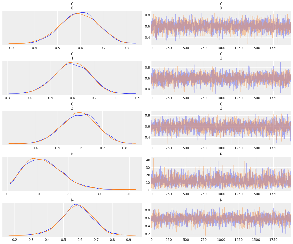
az.summary(mcmc5)
| mean | sd | hdi_3% | hdi_97% | mcse_mean | mcse_sd | ess_bulk | ess_tail | r_hat | |
|---|---|---|---|---|---|---|---|---|---|
| θ[0] | 0.595 | 0.081 | 0.442 | 0.743 | 0.001 | 0.001 | 4082.0 | 3197.0 | 1.0 |
| θ[1] | 0.598 | 0.080 | 0.441 | 0.737 | 0.001 | 0.001 | 4573.0 | 2541.0 | 1.0 |
| θ[2] | 0.597 | 0.079 | 0.456 | 0.747 | 0.001 | 0.001 | 4602.0 | 3073.0 | 1.0 |
| κ | 12.039 | 6.076 | 1.485 | 22.795 | 0.109 | 0.077 | 2685.0 | 1685.0 | 1.0 |
| μ | 0.582 | 0.098 | 0.399 | 0.767 | 0.002 | 0.001 | 3011.0 | 2157.0 | 1.0 |
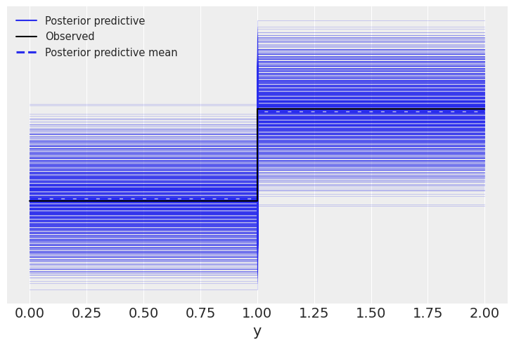
prior = Predictive(mcmc5.sampler.model, num_samples=10)
prior_p = prior(random.PRNGKey(seed), obs=data)

pred = Predictive(model=mcmc5.sampler.model, posterior_samples=mcmc5.get_samples(), return_sites=['y'])
post_p = pred(random.PRNGKey(seed))

samples = az.from_numpyro(mcmc5, prior=prior_p, posterior_predictive=post_p)
az.plot_ppc(samples, mean=True, observed=True, color='C0')
<AxesSubplot:xlabel='y'>
len(mcmc5.get_samples()['μ'])
4000
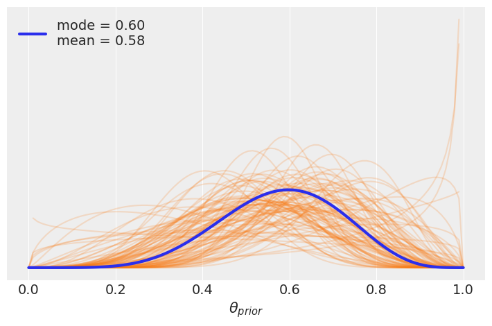
x = jnp.linspace(start=0, stop=1, num=100)
for i in random.randint(random.PRNGKey(1), shape=(100,), minval=0, maxval=len(mcmc5.get_samples()['μ'])):
    u = mcmc5.get_samples()['μ'][i]
    k = mcmc5.get_samples()['κ'][i]
    pdf = jnp.exp(dist.Beta(u*k, (1.0-u)*k).log_prob(x))
    plt.plot(x, pdf,  'C1', alpha=0.2)

u_mean = mcmc5.get_samples()['μ'].mean()
k_mean = mcmc5.get_samples()['κ'].mean()

distri = dist.Beta(u_mean*k_mean, (1.0-u_mean)*k_mean)
pdf = jnp.exp(distri.log_prob(x))
mode = x[jnp.argmax(pdf)]
mean = distri.mean
plt.plot(x, pdf, lw=3, label=f'mode = {mode:.2f}\nmean = {mean:.2f}')
plt.yticks([])

plt.legend()
plt.xlabel('$θ_{prior}$')
plt.tight_layout()
UserWarning: This figure was using constrained_layout, but that is incompatible with subplots_adjust and/or tight_layout; disabling constrained_layout.
cs_data = pd.read_csv('../data/chemical_shifts_theo_exp.csv')
diff = cs_data.theo.values - cs_data.exp.values
idx = pd.Categorical(cs_data['aa']).codes
groups = len(jnp.unique(idx))
cs_data.head()
| ID | aa | theo | exp | |
|---|---|---|---|---|
| 0 | 1BM8 | ILE | 61.18 | 58.27 |
| 1 | 1BM8 | TYR | 56.95 | 56.18 |
| 2 | 1BM8 | SER | 56.35 | 56.84 |
| 3 | 1BM8 | ALA | 51.96 | 51.01 |
| 4 | 1BM8 | ARG | 56.54 | 54.64 |
def model(obs=None):
    μ = numpyro.sample('μ', dist.Normal(loc=0., scale=10.), sample_shape=(groups,))
    σ = numpyro.sample('σ', dist.HalfNormal(scale=10.), sample_shape=(groups,))

    numpyro.sample('y', dist.Normal(loc=μ[idx], scale=σ[idx]), obs=obs, sample_shape=(len(cs_data),))


kernel = NUTS(model)
mcmc6 = MCMC(kernel, num_warmup=500, num_samples=500, num_chains=2)
mcmc6.run(random.PRNGKey(seed), obs=diff)
UserWarning: There are not enough devices to run parallel chains: expected 2 but got 1. Chains will be drawn sequentially. If you are running MCMC in CPU, consider using `numpyro.set_host_device_count(2)` at the beginning of your program. You can double-check how many devices are available in your system using `jax.local_device_count()`.
sample: 100%|███████████████████████████| 1000/1000 [00:03<00:00, 326.13it/s, 7 steps of size 4.78e-01. acc. prob=0.89]
sample: 100%|██████████████████████████| 1000/1000 [00:00<00:00, 2849.47it/s, 7 steps of size 4.74e-01. acc. prob=0.89]
def model(obs=None):
    # hyperpriors
    μ_μ = numpyro.sample('μ_μ', dist.Normal(loc=0., scale=10.))
    σ_μ = numpyro.sample('σ_μ', dist.HalfNormal(scale=10.))

    # priors
    μ = numpyro.sample('μ', dist.Normal(loc=μ_μ, scale=σ_μ), sample_shape=(groups,))
    σ = numpyro.sample('σ', dist.HalfNormal(scale=10.), sample_shape=(groups,))

    numpyro.sample('y', dist.Normal(loc=μ[idx], scale=σ[idx]), obs=obs, sample_shape=(len(cs_data),))


kernel = NUTS(model)
mcmc7 = MCMC(kernel, num_warmup=500, num_samples=500, num_chains=2)
mcmc7.run(random.PRNGKey(seed), obs=diff)
UserWarning: There are not enough devices to run parallel chains: expected 2 but got 1. Chains will be drawn sequentially. If you are running MCMC in CPU, consider using `numpyro.set_host_device_count(2)` at the beginning of your program. You can double-check how many devices are available in your system using `jax.local_device_count()`.
sample: 100%|███████████████████████████| 1000/1000 [00:03<00:00, 296.38it/s, 7 steps of size 4.91e-01. acc. prob=0.88]
sample: 100%|██████████████████████████| 1000/1000 [00:00<00:00, 2840.69it/s, 7 steps of size 5.15e-01. acc. prob=0.86]
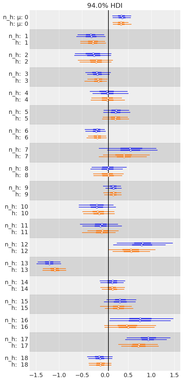
axes = az.plot_forest([mcmc6, mcmc7],
                         model_names=['n_h', 'h'],
                         var_names='μ', combined=False, colors='cycle')
y_lims = axes[0].get_ylim()
axes[0].vlines(jnp.mean(mcmc7.get_samples()['μ_μ']), color='k', *y_lims)
<matplotlib.collections.LineCollection at 0x12cb6c880>