
Chapter 5. Model Comparison
import os
import warnings

import arviz as az
import matplotlib.pyplot as plt
import pandas as pd
import seaborn as sns

import jax.numpy as jnp
from jax import random, vmap, local_device_count, pmap, lax, tree_map
from jax import nn as jnn
from jax.scipy import stats, special

import numpyro
import numpyro.distributions as dist
import numpyro.optim as optim

from numpyro.infer import MCMC, NUTS, HMC, Predictive
from numpyro.diagnostics import hpdi, print_summary
from numpyro.infer import Predictive, SVI, Trace_ELBO, init_to_value
from numpyro.infer.autoguide import AutoLaplaceApproximation

seed=1234

if "SVG" in os.environ:
    %config InlineBackend.figure_formats = ["svg"]
warnings.formatwarning = lambda message, category, *args, **kwargs: "{}: {}\n".format(
    category.__name__, message
)
az.style.use("arviz-darkgrid")
numpyro.set_platform("cpu") # or "gpu", "tpu" depending on system
numpyro.set_host_device_count(local_device_count())
# import pymc3 as pm
# import numpy as np
# import scipy.stats as stats
# import matplotlib.pyplot as plt
# import arviz as az
# az.style.use('arviz-darkgrid')
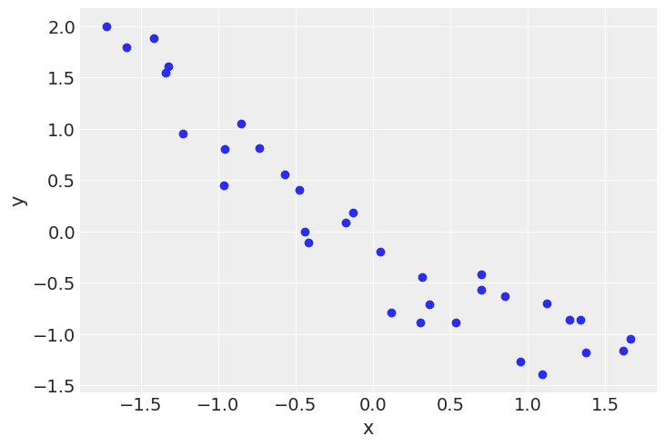
dummy_data = pd.read_csv('../data/dummy.csv', delimiter=' ', header=None, dtype=float)
x_1 = jnp.asarray(dummy_data)[:, 0]
y_1 = jnp.asarray(dummy_data)[:, 1]

order = 2
x_1p = jnp.vstack([x_1**i for i in range(1, order+1)])
x_1s = (x_1p - x_1p.mean(axis=1, keepdims=True)) / x_1p.std(axis=1, keepdims=True)
y_1s = (y_1 - y_1.mean()) / y_1.std()
plt.scatter(x_1s[0], y_1s)
plt.xlabel('x')
plt.ylabel('y')
Text(0, 0.5, 'y')
def model_l(obs=None):
    α = numpyro.sample('α', dist.Normal(loc=0, scale=1))
    β = numpyro.sample('β', dist.Normal(loc=0, scale=10))
    ϵ = numpyro.sample('ϵ', dist.HalfNormal(scale=5))

    μ = α + β * x_1s[0]

    y_pred = numpyro.sample('y_pred', dist.Normal(loc=μ, scale=ϵ), obs=obs)


kernel = NUTS(model_l)
mcmc_l = MCMC(kernel, num_warmup=500, num_samples=2000, num_chains=2, chain_method='sequential')
mcmc_l.run(random.PRNGKey(seed), obs=y_1s)

def model_p(obs=None):
    α = numpyro.sample('α', dist.Normal(loc=0, scale=1))
    β = numpyro.sample('β', dist.Normal(loc=0, scale=10), sample_shape=(order,))
    ϵ = numpyro.sample('ϵ', dist.HalfNormal(scale=5))

    μ = α + jnp.dot(β, x_1s)

    y_pred = numpyro.sample('y_pred', dist.Normal(loc=μ, scale=ϵ), obs=obs)


kernel = NUTS(model_p)
mcmc_p = MCMC(kernel, num_warmup=500, num_samples=2000, num_chains=2, chain_method='sequential')
mcmc_p.run(random.PRNGKey(seed), obs=y_1s)
sample: 100%|███████████████████████████| 2500/2500 [00:02<00:00, 915.45it/s, 3 steps of size 6.37e-01. acc. prob=0.95]
sample: 100%|██████████████████████████| 2500/2500 [00:00<00:00, 6931.30it/s, 3 steps of size 7.05e-01. acc. prob=0.93]
sample: 100%|██████████████████████████| 2500/2500 [00:02<00:00, 894.01it/s, 11 steps of size 2.61e-01. acc. prob=0.94]
sample: 100%|█████████████████████████| 2500/2500 [00:00<00:00, 6582.31it/s, 15 steps of size 2.86e-01. acc. prob=0.94]
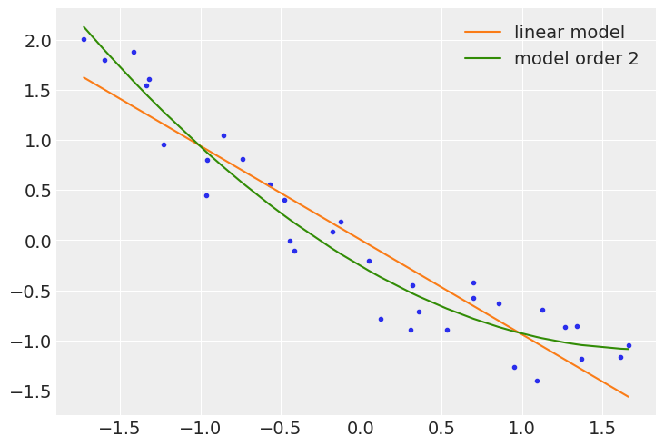
x_new = jnp.linspace(x_1s[0].min(), x_1s[0].max(), 100)

α_l_post = mcmc_l.get_samples()['α'].mean()
β_l_post = mcmc_l.get_samples()['β'].mean(axis=0)
y_l_post = α_l_post + β_l_post *  x_new

plt.plot(x_new, y_l_post, 'C1', label='linear model')

α_p_post = mcmc_p.get_samples()['α'].mean()
β_p_post = mcmc_p.get_samples()['β'].mean(axis=0)
idx = jnp.argsort(x_1s[0])
y_p_post = α_p_post + jnp.dot(β_p_post, x_1s)

plt.plot(x_1s[0][idx], y_p_post[idx], 'C2', label=f'model order {order}')

#α_p_post = trace_p['α'].mean()
#β_p_post = trace_p['β'].mean(axis=0)
#x_new_p = np.vstack([x_new**i for i in range(1, order+1)])
#y_p_post = α_p_post + np.dot(β_p_post, x_new_p)

plt.scatter(x_1s[0], y_1s, c='C0', marker='.')
plt.legend()
<matplotlib.legend.Legend at 0x135ca5790>
Posterior predictive checks
prior = Predictive(mcmc_l.sampler.model, num_samples=10)
prior_p = prior(random.PRNGKey(seed), obs=y_1s)

pred = Predictive(model=mcmc_l.sampler.model, posterior_samples=mcmc_l.get_samples(), return_sites=['y_pred'])
post_p = pred(random.PRNGKey(seed))
y_l = post_p['y_pred']

samples = az.from_numpyro(mcmc_l, posterior_predictive=post_p)
az.plot_ppc(samples, mean=True, observed=True, color='C0', alpha=0.01)
<AxesSubplot:xlabel='y_pred'>
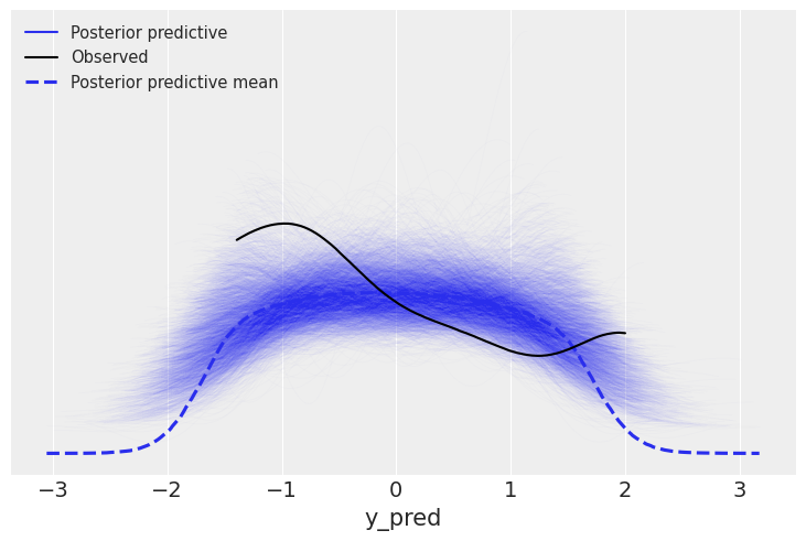
prior = Predictive(mcmc_p.sampler.model, num_samples=10)
prior_p = prior(random.PRNGKey(seed), obs=y_1s)

pred = Predictive(model=mcmc_p.sampler.model, posterior_samples=mcmc_p.get_samples(), return_sites=['y_pred'])
post_p = pred(random.PRNGKey(seed))
y_p = post_p['y_pred']

samples = az.from_numpyro(mcmc_p, posterior_predictive=post_p)
az.plot_ppc(samples, mean=True, observed=True, color='C0', alpha=0.01)
<AxesSubplot:xlabel='y_pred'>

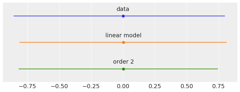
plt.figure(figsize=(8, 3))
data = [y_1s, y_l, y_p]
labels = ['data', 'linear model', 'order 2']
for i, d in enumerate(data):
    mean = d.mean()
    err = jnp.percentile(d, [25, 75])
    plt.errorbar(mean, -i, xerr=[[-err[0]], [err[1]]], fmt='o')
    plt.text(mean, -i+0.2, labels[i], ha='center', fontsize=14)
plt.ylim([-i-0.5, 0.5])
plt.yticks([])
([], [])
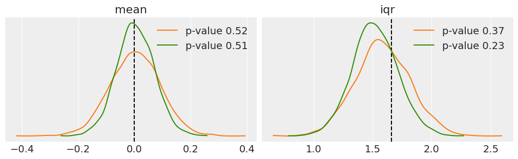
fig, ax = plt.subplots(1, 2, figsize=(10, 3), constrained_layout=True)


def iqr(x, a=0):
    return jnp.subtract(*jnp.percentile(x, [75, 25], axis=a))


for idx, func in enumerate([jnp.mean, iqr]):
    T_obs = func(y_1s)
    ax[idx].axvline(T_obs, 0, 1, color='k', ls='--')
    for d_sim, c in zip([y_l, y_p], ['C1', 'C2']):
        T_sim = func(d_sim, 1)
        p_value = jnp.mean(T_sim >= T_obs)
        az.plot_kde(T_sim, plot_kwargs={'color': c}, label=f'p-value {p_value:.2f}', ax=ax[idx])
    ax[idx].set_title(func.__name__)
    ax[idx].set_yticks([])
    ax[idx].legend()
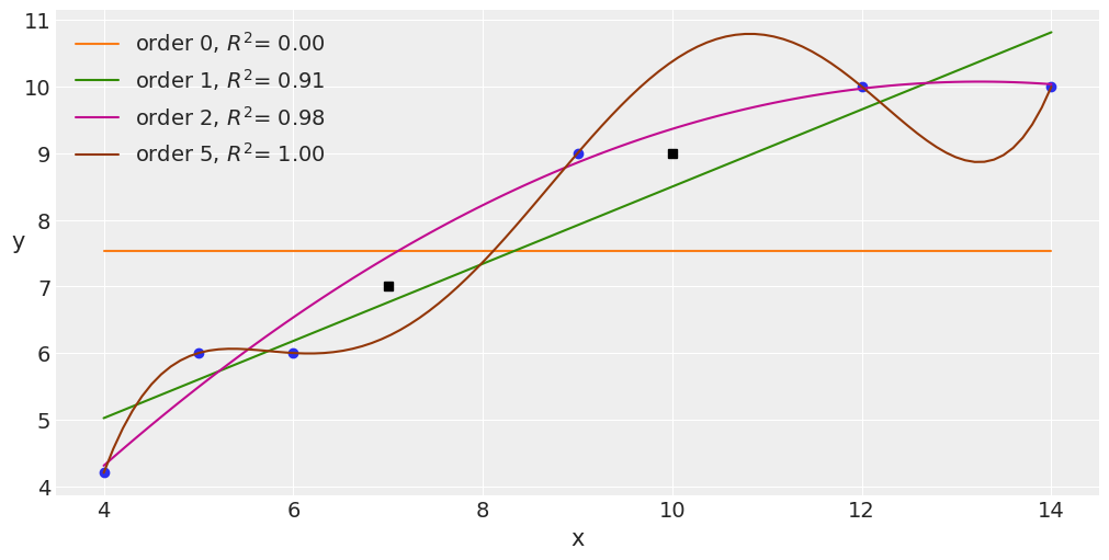
Occam’s razor – simplicity and accuracy
x = jnp.array([4., 5., 6., 9., 12, 14.])
y = jnp.array([4.2, 6., 6., 9., 10, 10.])

plt.figure(figsize=(10, 5))
orders = [0, 1, 2, 5]
plt.plot(x, y, 'o')
for i in orders:
    x_n = jnp.linspace(x.min(), x.max(), 100)
    coeffs = jnp.polyfit(x, y, deg=i)
    ffit = jnp.polyval(coeffs, x_n)

#     p = onp.poly1d(coeffs)
    yhat = jnp.polyval(coeffs, x)
#     yhat = p(x)
    ybar = jnp.mean(y)
    ssreg = jnp.sum((yhat-ybar)**2)
    sstot = jnp.sum((y - ybar)**2)
    r2 = ssreg / sstot

    plt.plot(x_n, ffit, label=f'order {i}, $R^2$= {r2:.2f}')

plt.legend(loc=2)
plt.xlabel('x')
plt.ylabel('y', rotation=0)
# plt.savefig('B11197_05_05.png', dpi=300)
plt.plot([10, 7], [9, 7], 'ks')
# plt.savefig('B11197_05_06.png', dpi=300)
[<matplotlib.lines.Line2D at 0x13bf93370>]
Computing information criteria with PyMC3
waic_l = az.waic(mcmc_l)
waic_l
Computed from 4000 by 33 log-likelihood matrix

          Estimate       SE
elpd_waic   -14.38     2.67
p_waic        2.44        -
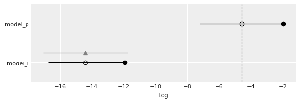
cmp_df = az.compare({'model_l':mcmc_l, 'model_p':mcmc_p},
                    method='BB-pseudo-BMA')
cmp_df
UserWarning: The default method used to estimate the weights for each model,has changed from BB-pseudo-BMA to stacking
| rank | loo | p_loo | d_loo | weight | se | dse | warning | loo_scale | |
|---|---|---|---|---|---|---|---|---|---|
| model_p | 0 | -4.579088 | 2.623271 | 0.000000 | 0.998345 | 2.625487 | 0.000000 | False | log |
| model_l | 1 | -14.409419 | 2.472847 | 9.830331 | 0.001655 | 2.363713 | 2.655246 | False | log |
az.plot_compare(cmp_df)
<AxesSubplot:xlabel='Log'>
Model Averaging
# TODO: figure out how to do this in numpyro
# w = 0.5
# y_lp = pm.sample_posterior_predictive_w([trace_l, trace_p],
#                                         samples=1000,
#                                         models=[model_l, model_p],
#                                         weights=[w, 1-w])
# _, ax = plt.subplots(figsize=(10, 6))
# az.plot_kde(y_l, plot_kwargs={'color': 'C1'}, label='linear model', ax=ax)
# az.plot_kde(y_p, plot_kwargs={'color': 'C2'}, label='order 2 model', ax=ax)
# az.plot_kde(y_lp['y_pred'], plot_kwargs={'color': 'C3'},
#            label='weighted model', ax=ax)

# plt.plot(y_1s, jnp.zeros_like(y_1s), '|', label='observed data')
# plt.yticks([])
# plt.legend()
# plt.savefig('B11197_05_09.png', dpi=300)
Bayes factors
coins = 30 # 300
heads = 9 # 90
y_d = jnp.repeat(jnp.array([0, 1]), jnp.array([coins-heads, heads]))
p = jnp.array([0.5, 0.5])
print(p)
model_index = dist.Categorical(probs=p).sample(key=random.PRNGKey(2), sample_shape=(10,))

m_0 = (4, 8)
m_1 = (8, 4)
checkeq = lax.eq(model_index, 0)
checkeq.astype(int)
print(checkeq.astype(int))
# m = lax.switch(checkeq, m_0, m_1)
[0.5 0.5]
[1 0 0 1 1 1 1 0 0 1]
# def model(obs=None):
#     p = jnp.array([0.5, 0.5])
#     model_index = numpyro.sample('model_index', dist.Categorical(probs=p))

#     m_0 = (4, 8)
#     m_1 = (8, 4)
#     checkeq = lax.eq(model_index, 0).astype(int)
#     m = lax.switch(checkeq, m_0, m_1)
# #     m = pm.math.switch(pm.math.eq(model_index, 0), m_0, m_1)

#     # a priori
#     θ = numpyro.sample('θ', dist.Beta(concentration1=m[0], concentration0=m[1]))
#     # likelihood
#     y = numpyro.sample('y', dist.Bernoulli(probs=θ), obs=obs)


# kernel = NUTS(model)
# mcmc_BF = MCMC(kernel, num_warmup=500, num_samples=2000, num_chains=2, chain_method='sequential')
# mcmc_BF.run(random.PRNGKey(seed), obs=y_d)

# az.plot_trace(mcmc_BF)
# with pm.Model() as model_BF:
#     p = np.array([0.5, 0.5])
#     model_index = pm.Categorical('model_index', p=p)

#     m_0 = (4, 8)
#     m_1 = (8, 4)
#     m = pm.math.switch(pm.math.eq(model_index, 0), m_0, m_1)

#     # a priori
#     θ = pm.Beta('θ', m[0], m[1])
#     # likelihood
#     y = pm.Bernoulli('y', θ, observed=y_d)

#     trace_BF = pm.sample(5000)
# az.plot_trace(trace_BF)
# plt.savefig('B11197_05_11.png', dpi=300)
# pM1 = mcmc_BF.get_samples()['model_index'].mean()
# pM0 = 1 - pM1
# BF = (pM0 / pM1) * (p[1] / p[0])
# BF
def model_BF_0(obs=None):
    θ = numpyro.sample('θ', dist.Beta(concentration1=4, concentration0=8))
    y = numpyro.sample('y', dist.Bernoulli(probs=θ), obs=obs)

kernel = NUTS(model_BF_0)
mcmc_BF_0 = MCMC(kernel, num_warmup=500, num_samples=2000, num_chains=2, chain_method='sequential')
mcmc_BF_0.run(random.PRNGKey(seed), obs=y_d)

def model_BF_1(obs=None):
    θ = numpyro.sample('θ', dist.Beta(concentration1=8, concentration0=4))
    y = numpyro.sample('y', dist.Bernoulli(probs=θ), obs=obs)

kernel = NUTS(model_BF_1)
mcmc_BF_1 = MCMC(kernel, num_warmup=500, num_samples=2000, num_chains=2, chain_method='sequential')
mcmc_BF_1.run(random.PRNGKey(seed), obs=y_d)
sample: 100%|███████████████████████████| 2500/2500 [00:02<00:00, 915.99it/s, 3 steps of size 9.87e-01. acc. prob=0.94]
sample: 100%|██████████████████████████| 2500/2500 [00:00<00:00, 4046.24it/s, 1 steps of size 1.03e+00. acc. prob=0.93]
sample: 100%|███████████████████████████| 2500/2500 [00:02<00:00, 915.59it/s, 3 steps of size 9.37e-01. acc. prob=0.94]
sample: 100%|██████████████████████████| 2500/2500 [00:00<00:00, 4153.99it/s, 1 steps of size 1.13e+00. acc. prob=0.89]
# https://forum.pyro.ai/t/mcmc-and-marginal-likelihood/2025
# model_BF_0.marginal_likelihood / model_BF_1.marginal_likelihood
Bayes factors and information criteria
traces = []
waics = []

for coins, heads in [(30, 9), (300, 90)]:
    y_d = jnp.repeat(jnp.array([0, 1]), jnp.array([coins-heads, heads]))
    for priors in [(4, 8), (8, 4)]:
        def model(obs=None): # with pm.Model() as model:
            θ = numpyro.sample('θ', dist.Beta(*priors))
            y = numpyro.sample('y', dist.Bernoulli(probs=θ), obs=obs)
#             trace = pm.sample(2000)
        kernel = NUTS(model)
        trace = MCMC(kernel, num_warmup=500, num_samples=2000, num_chains=2, chain_method='sequential')
        trace.run(random.PRNGKey(seed), obs=y_d)
        traces.append(trace)
        waics.append(az.waic(trace))
sample: 100%|███████████████████████████| 2500/2500 [00:02<00:00, 954.85it/s, 3 steps of size 9.87e-01. acc. prob=0.94]
sample: 100%|██████████████████████████| 2500/2500 [00:00<00:00, 7386.16it/s, 1 steps of size 1.03e+00. acc. prob=0.93]
sample: 100%|██████████████████████████| 2500/2500 [00:02<00:00, 1087.66it/s, 3 steps of size 9.37e-01. acc. prob=0.94]
sample: 100%|██████████████████████████| 2500/2500 [00:00<00:00, 7243.88it/s, 1 steps of size 1.13e+00. acc. prob=0.89]
sample: 100%|██████████████████████████| 2500/2500 [00:02<00:00, 1031.30it/s, 3 steps of size 9.27e-01. acc. prob=0.94]
sample: 100%|██████████████████████████| 2500/2500 [00:00<00:00, 6918.44it/s, 1 steps of size 1.32e+00. acc. prob=0.88]
sample: 100%|███████████████████████████| 2500/2500 [00:02<00:00, 964.63it/s, 3 steps of size 1.05e+00. acc. prob=0.94]
sample: 100%|██████████████████████████| 2500/2500 [00:00<00:00, 7002.64it/s, 3 steps of size 9.68e-01. acc. prob=0.92]
traces
[<numpyro.infer.mcmc.MCMC at 0x13bc96fa0>,
 <numpyro.infer.mcmc.MCMC at 0x13c9900a0>,
 <numpyro.infer.mcmc.MCMC at 0x13c3ea0a0>,
 <numpyro.infer.mcmc.MCMC at 0x13cdf9580>]
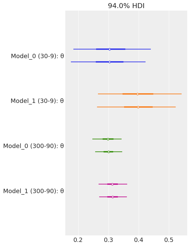
model_names = ['Model_0 (30-9)', 'Model_1 (30-9)',
               'Model_0 (300-90)', 'Model_1 (300-90)']

az.plot_forest(traces, model_names=model_names)
array([<AxesSubplot:title={'center':'94.0% HDI'}>], dtype=object)
waics
[Computed from 4000 by 30 log-likelihood matrix

           Estimate       SE
 elpd_waic   -19.01     2.14
 p_waic        0.68        -,
 Computed from 4000 by 30 log-likelihood matrix

           Estimate       SE
 elpd_waic   -19.59     1.08
 p_waic        0.63        -,
 Computed from 4000 by 300 log-likelihood matrix

           Estimate       SE
 elpd_waic  -184.16     6.80
 p_waic        0.90        -,
 Computed from 4000 by 300 log-likelihood matrix

           Estimate       SE
 elpd_waic  -184.26     6.26
 p_waic        0.88        -]
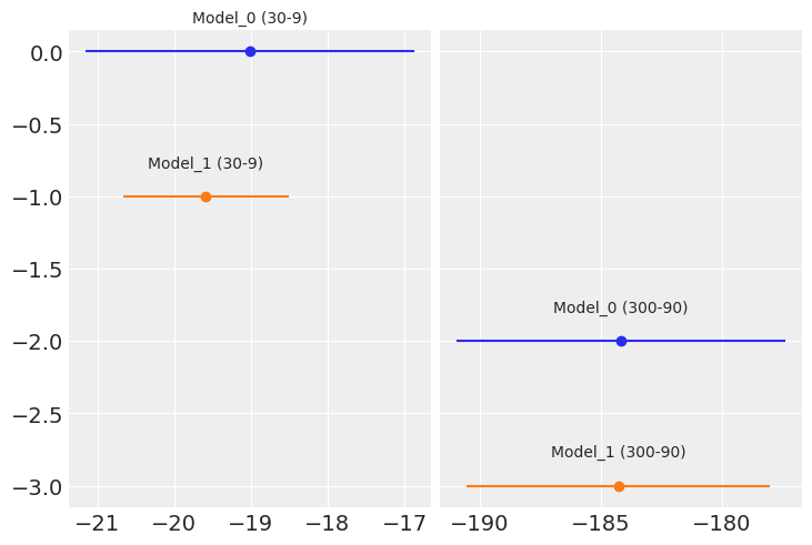
fig, ax = plt.subplots(1, 2, sharey=True)

labels = model_names
indices = [0, 0, 1, 1]
for i, (ind, d) in enumerate(zip(indices, waics)):
    mean = d.waic
    ax[ind].errorbar(mean, -i, xerr=d.waic_se, fmt='o')
    ax[ind].text(mean, -i+0.2, labels[i], ha='center')

# ax[0].set_xlim(30, 50)
# ax[1].set_xlim(330, 400)
# plt.ylim([-i-0.5, 0.5])
# plt.yticks([])
# plt.subplots_adjust(wspace=0.05)
# fig.text(0.5, 0, 'Deviance', ha='center', fontsize=14)
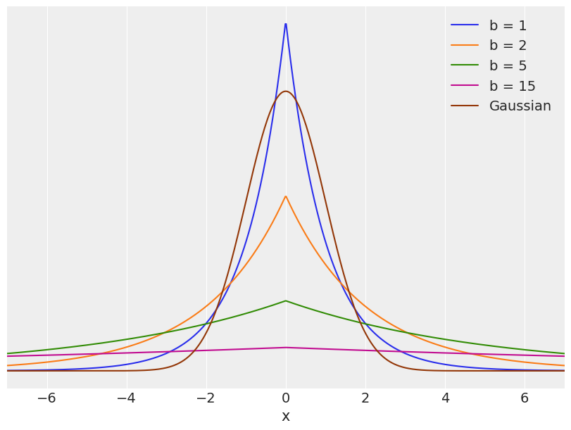
Regularizing priors
plt.figure(figsize=(8, 6))
x_values = jnp.linspace(-10, 10, 1000)
for df in [1, 2, 5, 15]:
#     distri = stats.laplace(scale=df)
    distri = dist.Laplace(scale=df)
    x_pdf = jnp.exp(distri.log_prob(x_values))
    plt.plot(x_values, x_pdf, label=f'b = {df}')

x_pdf = jnp.exp(dist.Normal().log_prob(x_values))
    #stats.norm.pdf(x_values)
plt.plot(x_values, x_pdf, label='Gaussian')
plt.xlabel('x')
plt.yticks([])
plt.legend()
plt.xlim(-7, 7)
(-7.0, 7.0)
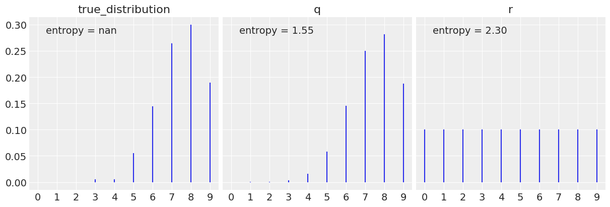
# x = range(0, 10)
x = jnp.arange(0, 10)
q = dist.Binomial(total_count=10, probs=0.75)
# r = random.randint(key=random.PRNGKey(0), shape=x, minval=0, maxval=10,)
r = dist.Uniform(low=0, high=10)
# data = stats.bernoulli.rvs(p=theta_real, size=trials)
# data = dist.Bernoulli(probs=theta_real).sample(random.PRNGKey(1), (trials,))

true_distribution = [list(q.sample(random.PRNGKey(i), (200,))).count(i) / 200 for i in x]

q_pmf = jnp.exp(q.log_prob(x))
r_pmf = jnp.exp(r.log_prob(x))

_, ax = plt.subplots(1, 3, figsize=(12, 4), sharey=True,
                     constrained_layout=True)

for idx, (dist, label) in enumerate(zip([true_distribution, q_pmf, r_pmf], ['true_distribution', 'q', 'r'])):
    h = -jnp.sum(jnp.array(dist) * jnp.log(jnp.array(dist))) # Entropy
    ax[idx].vlines(x, 0, dist, label=f'entropy = {h:.2f}')
    ax[idx].set_title(label)
    ax[idx].set_xticks(x)
    ax[idx].legend(loc=2, handlelength=0)
# import numpy as np
# np.random.seed(912)
# x = range(0, 10)
# q = scipy.stats.binom(10, 0.75)
# r = scipy.stats.randint(0, 10)

# true_distribution = [list(q.rvs(200)).count(i) / 200 for i in x]

# q_pmf = q.pmf(x)
# r_pmf = r.pmf(x)

# _, ax = plt.subplots(1, 3, figsize=(12, 4), sharey=True,
#                      constrained_layout=True)

# for idx, (distri, label) in enumerate(zip([true_distribution, q_pmf, r_pmf], ['true_distribution', 'q', 'r'])):
#     ax[idx].vlines(x, 0, dist, label=f'entropy = {scipy.stats.entropy(dist):.2f}')
#     print("X", dist)
#     print("XX", type(dist))
#     ax[idx].set_title(label)
#     ax[idx].set_xticks(x)
#     ax[idx].legend(loc=2, handlelength=0)

# plt.savefig('B11197_05_15.png', dpi=300)
# If qk is not None, then compute the Kullback-Leibler divergence S = sum(pk * log(pk / qk), axis=axis).
# H = -jnp.sum(jnp.array(dist) * jnp.log(jnp.array(dist))) # Entropy

def KLD(pk, qk, base=None, axis=0):

    if base is not None and base <= 0:
        raise ValueError("`base` must be a positive number or `None`.")

    pk = jnp.asarray(pk)
    pk = 1.0*pk / jnp.sum(pk, axis=axis, keepdims=True)
    if qk is None:
        vec = special.entr(pk)
    else:
        qk = jnp.asarray(qk)
        pk, qk = jnp.broadcast_arrays(pk, qk)
        qk = 1.0*qk / jnp.sum(qk, axis=axis, keepdims=True)
        vec = scipy.special.rel_entr(pk, qk)
    S = jnp.sum(vec, axis=axis)
    if base is not None:
        S /= jnp.log(base)
    return S

KLD(q_pmf, r_pmf)
DeviceArray(0.71549076, dtype=float32)
import scipy
scipy.stats.entropy(true_distribution, q_pmf), scipy.stats.entropy(true_distribution, r_pmf)
(0.0074029481416101415, 0.7618786232356769)
scipy.stats.entropy(r_pmf, q_pmf), scipy.stats.entropy(q_pmf, r_pmf)
(2.7569299, 0.71549076)